import geopandas as gpd
import pandas as pd
from shapely.geometry import LineString

# for interactive maps
import folium
from folium import Choropleth, Circle, Marker
from folium.plugins import HeatMap, MarkerCluster
import math
GeoDataFrame which has all capabilities of Pandas DataFrame
- Basic information (Gograhical data Frame)
gdf.info()
gdf.columns
gdf.shape
gdf.dtypes
- Geospatial-Attributes
gdf.geometry
gdf.crs
gdf.geom_type - provides geometry for each row (ponit, LineString, Polygon, etc.)
- Data Exploration:
gdf.head()
gdf.describe()
- Spatial Operation:
gdf.area
gdf.distance
gdf.buffer
- Plotting
gdf.plot()
data = gpd.read_file("C:\\Users\\Khurana_Kunal\\Downloads\\DEC_lands 2\\DEC_lands")data.head()| OBJECTID | CATEGORY | UNIT | FACILITY | CLASS | UMP | DESCRIPTIO | REGION | COUNTY | URL | SOURCE | UPDATE_ | OFFICE | ACRES | LANDS_UID | GREENCERT | SHAPE_AREA | SHAPE_LEN | geometry | |
|---|---|---|---|---|---|---|---|---|---|---|---|---|---|---|---|---|---|---|---|
| 0 | 1 | FOR PRES DET PAR | CFP | HANCOCK FP DETACHED PARCEL | WILD FOREST | None | DELAWARE COUNTY DETACHED PARCEL | 4 | DELAWARE | http://www.dec.ny.gov/ | DELAWARE RPP | 5/12 | STAMFORD | 738.620192 | 103 | N | 2.990365e+06 | 7927.662385 | POLYGON ((486093.245 4635308.586, 486787.235 4... |
| 1 | 2 | FOR PRES DET PAR | CFP | HANCOCK FP DETACHED PARCEL | WILD FOREST | None | DELAWARE COUNTY DETACHED PARCEL | 4 | DELAWARE | http://www.dec.ny.gov/ | DELAWARE RPP | 5/12 | STAMFORD | 282.553140 | 1218 | N | 1.143940e+06 | 4776.375600 | POLYGON ((491931.514 4637416.256, 491305.424 4... |
| 2 | 3 | FOR PRES DET PAR | CFP | HANCOCK FP DETACHED PARCEL | WILD FOREST | None | DELAWARE COUNTY DETACHED PARCEL | 4 | DELAWARE | http://www.dec.ny.gov/ | DELAWARE RPP | 5/12 | STAMFORD | 234.291262 | 1780 | N | 9.485476e+05 | 5783.070364 | POLYGON ((486000.287 4635834.453, 485007.550 4... |
| 3 | 4 | FOR PRES DET PAR | CFP | GREENE COUNTY FP DETACHED PARCEL | WILD FOREST | None | None | 4 | GREENE | http://www.dec.ny.gov/ | GREENE RPP | 5/12 | STAMFORD | 450.106464 | 2060 | N | 1.822293e+06 | 7021.644833 | POLYGON ((541716.775 4675243.268, 541217.579 4... |
| 4 | 6 | FOREST PRESERVE | AFP | SARANAC LAKES WILD FOREST | WILD FOREST | SARANAC LAKES | None | 5 | ESSEX | http://www.dec.ny.gov/lands/22593.html | DECRP, ESSEX RPP | 12/96 | RAY BROOK | 69.702387 | 1517 | N | 2.821959e+05 | 2663.909932 | POLYGON ((583896.043 4909643.187, 583891.200 4... |
data_selected = data.loc[:, ['CLASS', 'COUNTY', 'geometry']].copy()data_selected.CLASS.value_counts()CLASS
WILD FOREST 965
INTENSIVE USE 108
PRIMITIVE 60
WILDERNESS 52
ADMINISTRATIVE 17
UNCLASSIFIED 7
HISTORIC 5
PRIMITIVE BICYCLE CORRIDOR 4
CANOE AREA 1
Name: count, dtype: int64# select lands under 'wild forest' or 'wilderness' category
wild_lands = data_selected.loc[data_selected.CLASS.isin(['WILD FOREST', 'WILDERNESS'])].copy()
wild_lands.head()| CLASS | COUNTY | geometry | |
|---|---|---|---|
| 0 | WILD FOREST | DELAWARE | POLYGON ((486093.245 4635308.586, 486787.235 4... |
| 1 | WILD FOREST | DELAWARE | POLYGON ((491931.514 4637416.256, 491305.424 4... |
| 2 | WILD FOREST | DELAWARE | POLYGON ((486000.287 4635834.453, 485007.550 4... |
| 3 | WILD FOREST | GREENE | POLYGON ((541716.775 4675243.268, 541217.579 4... |
| 4 | WILD FOREST | ESSEX | POLYGON ((583896.043 4909643.187, 583891.200 4... |
wild_lands.plot()<Axes: >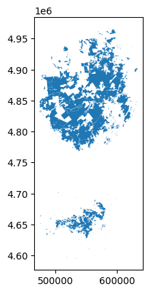
wild_lands.geometry.head()0 POLYGON ((486093.245 4635308.586, 486787.235 4...
1 POLYGON ((491931.514 4637416.256, 491305.424 4...
2 POLYGON ((486000.287 4635834.453, 485007.550 4...
3 POLYGON ((541716.775 4675243.268, 541217.579 4...
4 POLYGON ((583896.043 4909643.187, 583891.200 4...
Name: geometry, dtype: geometryworld_filepath ='geopandas\\ne_110m_admin_0_countries\\ne_110m_admin_0_countries.shx'
world = gpd.read_file(world_filepath)
world.head()| featurecla | scalerank | LABELRANK | SOVEREIGNT | SOV_A3 | ADM0_DIF | LEVEL | TYPE | TLC | ADMIN | ... | FCLASS_TR | FCLASS_ID | FCLASS_PL | FCLASS_GR | FCLASS_IT | FCLASS_NL | FCLASS_SE | FCLASS_BD | FCLASS_UA | geometry | |
|---|---|---|---|---|---|---|---|---|---|---|---|---|---|---|---|---|---|---|---|---|---|
| 0 | Admin-0 country | 1 | 6 | Fiji | FJI | 0 | 2 | Sovereign country | 1 | Fiji | ... | None | None | None | None | None | None | None | None | None | MULTIPOLYGON (((180.00000 -16.06713, 180.00000... |
| 1 | Admin-0 country | 1 | 3 | United Republic of Tanzania | TZA | 0 | 2 | Sovereign country | 1 | United Republic of Tanzania | ... | None | None | None | None | None | None | None | None | None | POLYGON ((33.90371 -0.95000, 34.07262 -1.05982... |
| 2 | Admin-0 country | 1 | 7 | Western Sahara | SAH | 0 | 2 | Indeterminate | 1 | Western Sahara | ... | Unrecognized | Unrecognized | Unrecognized | None | None | Unrecognized | None | None | None | POLYGON ((-8.66559 27.65643, -8.66512 27.58948... |
| 3 | Admin-0 country | 1 | 2 | Canada | CAN | 0 | 2 | Sovereign country | 1 | Canada | ... | None | None | None | None | None | None | None | None | None | MULTIPOLYGON (((-122.84000 49.00000, -122.9742... |
| 4 | Admin-0 country | 1 | 2 | United States of America | US1 | 1 | 2 | Country | 1 | United States of America | ... | None | None | None | None | None | None | None | None | None | MULTIPOLYGON (((-122.84000 49.00000, -120.0000... |
5 rows × 169 columns
ax = world.plot()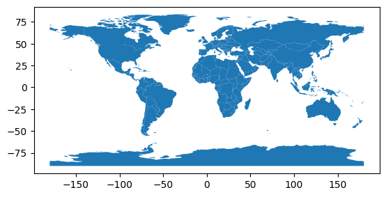
#plotting a map with coordinates
ax = world.plot(figsize=(20,20), color='whitesmoke', linestyle=':', edgecolor='black')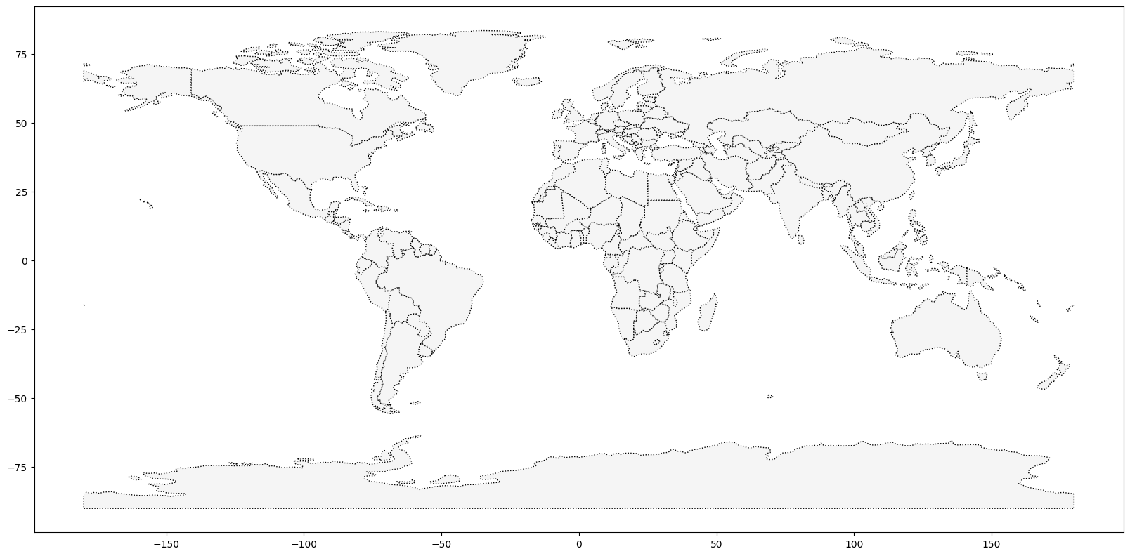
PHL_loans = data.loc[data.COUNTY=="Philippines"].copy()print(world.columns)Index(['featurecla', 'scalerank', 'LABELRANK', 'SOVEREIGNT', 'SOV_A3',
'ADM0_DIF', 'LEVEL', 'TYPE', 'TLC', 'ADMIN',
...
'FCLASS_TR', 'FCLASS_ID', 'FCLASS_PL', 'FCLASS_GR', 'FCLASS_IT',
'FCLASS_NL', 'FCLASS_SE', 'FCLASS_BD', 'FCLASS_UA', 'geometry'],
dtype='object', length=169)world.info()<class 'geopandas.geodataframe.GeoDataFrame'>
RangeIndex: 177 entries, 0 to 176
Columns: 169 entries, featurecla to geometry
dtypes: float64(6), geometry(1), int64(25), object(137)
memory usage: 233.8+ KBworld.head()| featurecla | scalerank | LABELRANK | SOVEREIGNT | SOV_A3 | ADM0_DIF | LEVEL | TYPE | TLC | ADMIN | ... | FCLASS_TR | FCLASS_ID | FCLASS_PL | FCLASS_GR | FCLASS_IT | FCLASS_NL | FCLASS_SE | FCLASS_BD | FCLASS_UA | geometry | |
|---|---|---|---|---|---|---|---|---|---|---|---|---|---|---|---|---|---|---|---|---|---|
| 0 | Admin-0 country | 1 | 6 | Fiji | FJI | 0 | 2 | Sovereign country | 1 | Fiji | ... | None | None | None | None | None | None | None | None | None | MULTIPOLYGON (((180.00000 -16.06713, 180.00000... |
| 1 | Admin-0 country | 1 | 3 | United Republic of Tanzania | TZA | 0 | 2 | Sovereign country | 1 | United Republic of Tanzania | ... | None | None | None | None | None | None | None | None | None | POLYGON ((33.90371 -0.95000, 34.07262 -1.05982... |
| 2 | Admin-0 country | 1 | 7 | Western Sahara | SAH | 0 | 2 | Indeterminate | 1 | Western Sahara | ... | Unrecognized | Unrecognized | Unrecognized | None | None | Unrecognized | None | None | None | POLYGON ((-8.66559 27.65643, -8.66512 27.58948... |
| 3 | Admin-0 country | 1 | 2 | Canada | CAN | 0 | 2 | Sovereign country | 1 | Canada | ... | None | None | None | None | None | None | None | None | None | MULTIPOLYGON (((-122.84000 49.00000, -122.9742... |
| 4 | Admin-0 country | 1 | 2 | United States of America | US1 | 1 | 2 | Country | 1 | United States of America | ... | None | None | None | None | None | None | None | None | None | MULTIPOLYGON (((-122.84000 49.00000, -120.0000... |
5 rows × 169 columns
Coordinate Reference Systems
- shape file imports CRS automatically
- settings (DataFrame uses EPSG 32630; csv file uses EPSG 4326)
facilities_df = pd.read_csv('geopandas\health_facilities.csv')

# convert to GeoDataFrame
facilities = gpd.GeoDataFrame(facilities_df, geometry = gpd.points_from_xy
                              (facilities_df.Longitude, facilities_df.Latitude))

# set CRS
facilities.crs = ('epsg:4326')

#view first 5 rows
facilities.head()| Region | District | FacilityName | Type | Town | Ownership | Latitude | Longitude | geometry | |
|---|---|---|---|---|---|---|---|---|---|
| 0 | Ashanti | Offinso North | A.M.E Zion Clinic | Clinic | Afrancho | CHAG | 7.40801 | -1.96317 | POINT (-1.96317 7.40801) |
| 1 | Ashanti | Bekwai Municipal | Abenkyiman Clinic | Clinic | Anwiankwanta | Private | 6.46312 | -1.58592 | POINT (-1.58592 6.46312) |
| 2 | Ashanti | Adansi North | Aboabo Health Centre | Health Centre | Aboabo No 2 | Government | 6.22393 | -1.34982 | POINT (-1.34982 6.22393) |
| 3 | Ashanti | Afigya-Kwabre | Aboabogya Health Centre | Health Centre | Aboabogya | Government | 6.84177 | -1.61098 | POINT (-1.61098 6.84177) |
| 4 | Ashanti | Kwabre | Aboaso Health Centre | Health Centre | Aboaso | Government | 6.84177 | -1.61098 | POINT (-1.61098 6.84177) |
# plotting facilities of Ghana on world map
ax = world.plot(figsize=(20,20), color='whitesmoke', linestyle=':', edgecolor='black')
facilities.to_crs(epsg=4326).plot(markersize=.25, ax=ax)
C:\Users\Khurana_Kunal\anaconda3\Lib\site-packages\shapely\measurement.py:103: RuntimeWarning: invalid value encountered in bounds
return lib.bounds(geometry_arr, out=out, **kwargs)<Axes: >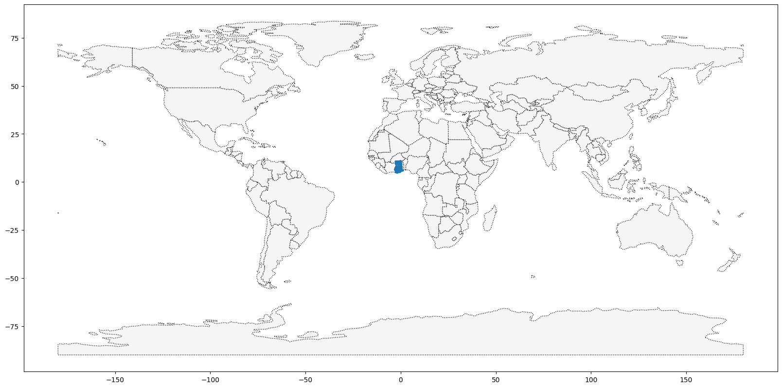
#get the x coordinates of each point
facilities.geometry.head().x
0 -1.96317
1 -1.58592
2 -1.34982
3 -1.61098
4 -1.61098
dtype: float64birds_df = pd.read_csv("data_for_all_courses\purple_martin.csv")
birds_df.head()| timestamp | location-long | location-lat | tag-local-identifier | |
|---|---|---|---|---|
| 0 | 2014-08-15 05:56:00 | -88.146014 | 17.513049 | 30448 |
| 1 | 2014-09-01 05:59:00 | -85.243501 | 13.095782 | 30448 |
| 2 | 2014-10-30 23:58:00 | -62.906089 | -7.852436 | 30448 |
| 3 | 2014-11-15 04:59:00 | -61.776826 | -11.723898 | 30448 |
| 4 | 2014-11-30 09:59:00 | -61.241538 | -11.612237 | 30448 |
print(f"There are {birds_df['tag-local-identifier'].nunique()} different birds in the dataset.")There are 11 different birds in the dataset.birds = gpd.GeoDataFrame(birds_df,
geometry = gpd.points_from_xy(birds_df["location-long"],
birds_df['location-lat']))
birds.head()| timestamp | location-long | location-lat | tag-local-identifier | geometry | |
|---|---|---|---|---|---|
| 0 | 2014-08-15 05:56:00 | -88.146014 | 17.513049 | 30448 | POINT (-88.14601 17.51305) |
| 1 | 2014-09-01 05:59:00 | -85.243501 | 13.095782 | 30448 | POINT (-85.24350 13.09578) |
| 2 | 2014-10-30 23:58:00 | -62.906089 | -7.852436 | 30448 | POINT (-62.90609 -7.85244) |
| 3 | 2014-11-15 04:59:00 | -61.776826 | -11.723898 | 30448 | POINT (-61.77683 -11.72390) |
| 4 | 2014-11-30 09:59:00 | -61.241538 | -11.612237 | 30448 | POINT (-61.24154 -11.61224) |
# set the CRS

birds.crs = ('epsg:4326')
# plot the data
americas = world.loc[world['CONTINENT'].isin(['North America', 'South America',])]
americas.head()| featurecla | scalerank | LABELRANK | SOVEREIGNT | SOV_A3 | ADM0_DIF | LEVEL | TYPE | TLC | ADMIN | ... | FCLASS_TR | FCLASS_ID | FCLASS_PL | FCLASS_GR | FCLASS_IT | FCLASS_NL | FCLASS_SE | FCLASS_BD | FCLASS_UA | geometry | |
|---|---|---|---|---|---|---|---|---|---|---|---|---|---|---|---|---|---|---|---|---|---|
| 3 | Admin-0 country | 1 | 2 | Canada | CAN | 0 | 2 | Sovereign country | 1 | Canada | ... | None | None | None | None | None | None | None | None | None | MULTIPOLYGON (((-122.84000 49.00000, -122.9742... |
| 4 | Admin-0 country | 1 | 2 | United States of America | US1 | 1 | 2 | Country | 1 | United States of America | ... | None | None | None | None | None | None | None | None | None | MULTIPOLYGON (((-122.84000 49.00000, -120.0000... |
| 9 | Admin-0 country | 1 | 2 | Argentina | ARG | 0 | 2 | Sovereign country | 1 | Argentina | ... | None | None | None | None | None | None | None | None | None | MULTIPOLYGON (((-68.63401 -52.63637, -68.25000... |
| 10 | Admin-0 country | 1 | 2 | Chile | CHL | 0 | 2 | Sovereign country | 1 | Chile | ... | None | None | None | None | None | None | None | None | None | MULTIPOLYGON (((-68.63401 -52.63637, -68.63335... |
| 16 | Admin-0 country | 1 | 5 | Haiti | HTI | 0 | 2 | Sovereign country | 1 | Haiti | ... | None | None | None | None | None | None | None | None | None | POLYGON ((-71.71236 19.71446, -71.62487 19.169... |
5 rows × 169 columns
world.head()| featurecla | scalerank | LABELRANK | SOVEREIGNT | SOV_A3 | ADM0_DIF | LEVEL | TYPE | TLC | ADMIN | ... | FCLASS_TR | FCLASS_ID | FCLASS_PL | FCLASS_GR | FCLASS_IT | FCLASS_NL | FCLASS_SE | FCLASS_BD | FCLASS_UA | geometry | |
|---|---|---|---|---|---|---|---|---|---|---|---|---|---|---|---|---|---|---|---|---|---|
| 0 | Admin-0 country | 1 | 6 | Fiji | FJI | 0 | 2 | Sovereign country | 1 | Fiji | ... | None | None | None | None | None | None | None | None | None | MULTIPOLYGON (((180.00000 -16.06713, 180.00000... |
| 1 | Admin-0 country | 1 | 3 | United Republic of Tanzania | TZA | 0 | 2 | Sovereign country | 1 | United Republic of Tanzania | ... | None | None | None | None | None | None | None | None | None | POLYGON ((33.90371 -0.95000, 34.07262 -1.05982... |
| 2 | Admin-0 country | 1 | 7 | Western Sahara | SAH | 0 | 2 | Indeterminate | 1 | Western Sahara | ... | Unrecognized | Unrecognized | Unrecognized | None | None | Unrecognized | None | None | None | POLYGON ((-8.66559 27.65643, -8.66512 27.58948... |
| 3 | Admin-0 country | 1 | 2 | Canada | CAN | 0 | 2 | Sovereign country | 1 | Canada | ... | None | None | None | None | None | None | None | None | None | MULTIPOLYGON (((-122.84000 49.00000, -122.9742... |
| 4 | Admin-0 country | 1 | 2 | United States of America | US1 | 1 | 2 | Country | 1 | United States of America | ... | None | None | None | None | None | None | None | None | None | MULTIPOLYGON (((-122.84000 49.00000, -120.0000... |
5 rows × 169 columns
# checking for all the columns in a data frame with for loop
for column in world.columns:
    print(column)
featurecla
scalerank
LABELRANK
SOVEREIGNT
SOV_A3
ADM0_DIF
LEVEL
TYPE
TLC
ADMIN
ADM0_A3
GEOU_DIF
GEOUNIT
GU_A3
SU_DIF
SUBUNIT
SU_A3
BRK_DIFF
NAME
NAME_LONG
BRK_A3
BRK_NAME
BRK_GROUP
ABBREV
POSTAL
FORMAL_EN
FORMAL_FR
NAME_CIAWF
NOTE_ADM0
NOTE_BRK
NAME_SORT
NAME_ALT
MAPCOLOR7
MAPCOLOR8
MAPCOLOR9
MAPCOLOR13
POP_EST
POP_RANK
POP_YEAR
GDP_MD
GDP_YEAR
ECONOMY
INCOME_GRP
FIPS_10
ISO_A2
ISO_A2_EH
ISO_A3
ISO_A3_EH
ISO_N3
ISO_N3_EH
UN_A3
WB_A2
WB_A3
WOE_ID
WOE_ID_EH
WOE_NOTE
ADM0_ISO
ADM0_DIFF
ADM0_TLC
ADM0_A3_US
ADM0_A3_FR
ADM0_A3_RU
ADM0_A3_ES
ADM0_A3_CN
ADM0_A3_TW
ADM0_A3_IN
ADM0_A3_NP
ADM0_A3_PK
ADM0_A3_DE
ADM0_A3_GB
ADM0_A3_BR
ADM0_A3_IL
ADM0_A3_PS
ADM0_A3_SA
ADM0_A3_EG
ADM0_A3_MA
ADM0_A3_PT
ADM0_A3_AR
ADM0_A3_JP
ADM0_A3_KO
ADM0_A3_VN
ADM0_A3_TR
ADM0_A3_ID
ADM0_A3_PL
ADM0_A3_GR
ADM0_A3_IT
ADM0_A3_NL
ADM0_A3_SE
ADM0_A3_BD
ADM0_A3_UA
ADM0_A3_UN
ADM0_A3_WB
CONTINENT
REGION_UN
SUBREGION
REGION_WB
NAME_LEN
LONG_LEN
ABBREV_LEN
TINY
HOMEPART
MIN_ZOOM
MIN_LABEL
MAX_LABEL
LABEL_X
LABEL_Y
NE_ID
WIKIDATAID
NAME_AR
NAME_BN
NAME_DE
NAME_EN
NAME_ES
NAME_FA
NAME_FR
NAME_EL
NAME_HE
NAME_HI
NAME_HU
NAME_ID
NAME_IT
NAME_JA
NAME_KO
NAME_NL
NAME_PL
NAME_PT
NAME_RU
NAME_SV
NAME_TR
NAME_UK
NAME_UR
NAME_VI
NAME_ZH
NAME_ZHT
FCLASS_ISO
TLC_DIFF
FCLASS_TLC
FCLASS_US
FCLASS_FR
FCLASS_RU
FCLASS_ES
FCLASS_CN
FCLASS_TW
FCLASS_IN
FCLASS_NP
FCLASS_PK
FCLASS_DE
FCLASS_GB
FCLASS_BR
FCLASS_IL
FCLASS_PS
FCLASS_SA
FCLASS_EG
FCLASS_MA
FCLASS_PT
FCLASS_AR
FCLASS_JP
FCLASS_KO
FCLASS_VN
FCLASS_TR
FCLASS_ID
FCLASS_PL
FCLASS_GR
FCLASS_IT
FCLASS_NL
FCLASS_SE
FCLASS_BD
FCLASS_UA
geometry# plot americas
ax_americas = americas.plot(figsize=(10,10), color='whitesmoke', linestyle=':', edgecolor='black')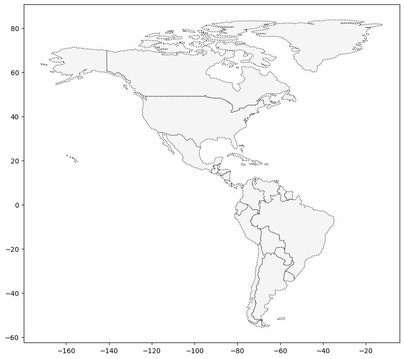
Starting and end journey of birds
# GeoDataFrame showing path for each bird
path_df = birds.groupby("tag-local-identifier")['geometry'].apply(list).apply(lambda x: LineString(x)).reset_index()
path_gdf = gpd.GeoDataFrame(path_df, geometry = path_df.geometry)
path_gdf.crs = ('epsg:4326')

# GeoDataFrame showing starting point for each bird
start_df = birds.groupby("tag-local-identifier")['geometry'].apply(list).apply(lambda x: x[0]).reset_index()
start_gdf = gpd.GeoDataFrame(start_df, geometry = start_df.geometry)
start_gdf.crs = ('epsg:4326')

# Show first five rows of GeoDataFrame
start_gdf.head()| tag-local-identifier | geometry | |
|---|---|---|
| 0 | 30048 | POINT (-90.12992 20.73242) |
| 1 | 30054 | POINT (-93.60861 46.50563) |
| 2 | 30198 | POINT (-80.31036 25.92545) |
| 3 | 30263 | POINT (-76.78146 42.99209) |
| 4 | 30275 | POINT (-76.78213 42.99207) |
# end point of each bird
end_df = birds.groupby("tag-local-identifier")['geometry'].apply(list).apply(lambda x: x[-1]).reset_index()
end_gdf = gpd.GeoDataFrame(end_df, geometry = end_df.geometry)
end_gdf.crs = ('epsg:4326')
# plot americas
ax_americas = americas.plot(figsize=(10,10), color='whitesmoke', linestyle=':', edgecolor='black')
start_gdf.plot(ax = ax_americas, color = 'red', markersize = 10)
path_gdf.plot(ax = ax_americas, cmap = 'tab20b', linestyle= '-', linewidth = 1, zorder = 1)
end_gdf.plot(ax = ax_americas, color = 'blue', markersize = 10)<Axes: >
# no file found; gives 'Driver Error' - à voir plustard
protected_filepath = 'data_for_all_courses/add_0.shp'
protected_area = gpd.read_file(protected_filepath)
Interactive maps
# Create a map
montréal_1 = folium.Map(location=[45.50, -73.56], tiles='openstreetmap', zoom_start=10)


# Display the map
montréal_1
Make this Notebook Trusted to load map: File -> Trust Notebook
# crimes

crimes = pd.read_csv("data_for_all_courses\crime.csv", encoding = 'latin-1')
crimes.describe()
| OFFENSE_CODE | YEAR | MONTH | HOUR | Lat | Long | |
|---|---|---|---|---|---|---|
| count | 319073.000000 | 319073.000000 | 319073.000000 | 319073.000000 | 299074.000000 | 299074.000000 |
| mean | 2317.546956 | 2016.560586 | 6.609719 | 13.118205 | 42.214381 | -70.908272 |
| std | 1185.285543 | 0.996344 | 3.273691 | 6.294205 | 2.159766 | 3.493618 |
| min | 111.000000 | 2015.000000 | 1.000000 | 0.000000 | -1.000000 | -71.178674 |
| 25% | 1001.000000 | 2016.000000 | 4.000000 | 9.000000 | 42.297442 | -71.097135 |
| 50% | 2907.000000 | 2017.000000 | 7.000000 | 14.000000 | 42.325538 | -71.077524 |
| 75% | 3201.000000 | 2017.000000 | 9.000000 | 18.000000 | 42.348624 | -71.062467 |
| max | 3831.000000 | 2018.000000 | 12.000000 | 23.000000 | 42.395042 | -1.000000 |
crimes.head()| INCIDENT_NUMBER | OFFENSE_CODE | OFFENSE_CODE_GROUP | OFFENSE_DESCRIPTION | DISTRICT | REPORTING_AREA | SHOOTING | OCCURRED_ON_DATE | YEAR | MONTH | DAY_OF_WEEK | HOUR | UCR_PART | STREET | Lat | Long | Location | |
|---|---|---|---|---|---|---|---|---|---|---|---|---|---|---|---|---|---|
| 0 | I182070945 | 619 | Larceny | LARCENY ALL OTHERS | D14 | 808 | NaN | 2018-09-02 13:00:00 | 2018 | 9 | Sunday | 13 | Part One | LINCOLN ST | 42.357791 | -71.139371 | (42.35779134, -71.13937053) |
| 1 | I182070943 | 1402 | Vandalism | VANDALISM | C11 | 347 | NaN | 2018-08-21 00:00:00 | 2018 | 8 | Tuesday | 0 | Part Two | HECLA ST | 42.306821 | -71.060300 | (42.30682138, -71.06030035) |
| 2 | I182070941 | 3410 | Towed | TOWED MOTOR VEHICLE | D4 | 151 | NaN | 2018-09-03 19:27:00 | 2018 | 9 | Monday | 19 | Part Three | CAZENOVE ST | 42.346589 | -71.072429 | (42.34658879, -71.07242943) |
| 3 | I182070940 | 3114 | Investigate Property | INVESTIGATE PROPERTY | D4 | 272 | NaN | 2018-09-03 21:16:00 | 2018 | 9 | Monday | 21 | Part Three | NEWCOMB ST | 42.334182 | -71.078664 | (42.33418175, -71.07866441) |
| 4 | I182070938 | 3114 | Investigate Property | INVESTIGATE PROPERTY | B3 | 421 | NaN | 2018-09-03 21:05:00 | 2018 | 9 | Monday | 21 | Part Three | DELHI ST | 42.275365 | -71.090361 | (42.27536542, -71.09036101) |
# drop missing locations
crimes.dropna(subset= ['Lat', 'Long', 'DISTRICT'], inplace = True)
# focus on major crimes
crimes = crimes[crimes.OFFENSE_CODE_GROUP.isin([
'Larceny', 'Auto Theft', 'Robbery', 'Larceny From Motor Vehicle', 'Residential Burglary',
'Simple Assault', 'Harassment', 'Ballistics', 'Aggravated Assault', 'Other Burglary',
'Arson', 'Commercial Burglary'
])]
crimes = crimes[crimes.YEAR>=2018]
crimes.head()| INCIDENT_NUMBER | OFFENSE_CODE | OFFENSE_CODE_GROUP | OFFENSE_DESCRIPTION | DISTRICT | REPORTING_AREA | SHOOTING | OCCURRED_ON_DATE | YEAR | MONTH | DAY_OF_WEEK | HOUR | UCR_PART | STREET | Lat | Long | Location | |
|---|---|---|---|---|---|---|---|---|---|---|---|---|---|---|---|---|---|
| 0 | I182070945 | 619 | Larceny | LARCENY ALL OTHERS | D14 | 808 | NaN | 2018-09-02 13:00:00 | 2018 | 9 | Sunday | 13 | Part One | LINCOLN ST | 42.357791 | -71.139371 | (42.35779134, -71.13937053) |
| 6 | I182070933 | 724 | Auto Theft | AUTO THEFT | B2 | 330 | NaN | 2018-09-03 21:25:00 | 2018 | 9 | Monday | 21 | Part One | NORMANDY ST | 42.306072 | -71.082733 | (42.30607218, -71.08273260) |
| 8 | I182070931 | 301 | Robbery | ROBBERY - STREET | C6 | 177 | NaN | 2018-09-03 20:48:00 | 2018 | 9 | Monday | 20 | Part One | MASSACHUSETTS AVE | 42.331521 | -71.070853 | (42.33152148, -71.07085307) |
| 19 | I182070915 | 614 | Larceny From Motor Vehicle | LARCENY THEFT FROM MV - NON-ACCESSORY | B2 | 181 | NaN | 2018-09-02 18:00:00 | 2018 | 9 | Sunday | 18 | Part One | SHIRLEY ST | 42.325695 | -71.068168 | (42.32569490, -71.06816778) |
| 24 | I182070908 | 522 | Residential Burglary | BURGLARY - RESIDENTIAL - NO FORCE | B2 | 911 | NaN | 2018-09-03 18:38:00 | 2018 | 9 | Monday | 18 | Part One | ANNUNCIATION RD | 42.335062 | -71.093168 | (42.33506218, -71.09316781) |
# crimes between 9 to 18

daytime_robberies = crimes[((crimes.OFFENSE_CODE_GROUP == 'Robbery') &
                            crimes.HOUR.isin(range(9,18)))]
# create a map
map2 = folium.Map(location=[42.32,-71.0589], tiles='openstreetmap', zoom_start=13)
# add points
for idx, row in daytime_robberies.iterrows():
Marker([row['Lat'], row['Long']]).add_to(map2)
# display
map2Make this Notebook Trusted to load map: File -> Trust Notebook
folium.plugin.MarkerCluster
# plotting points
m_3 = folium.Map(location= [42.32,-71.0589], tiles='cartodbpositron', zoom_start=13)

# add points
mc = MarkerCluster()
for idx, row in daytime_robberies.iterrows():
    if not math.isnan(row['Long']) and not math.isnan(row['Lat']):
        mc.add_child(Marker([row['Lat'], row['Long']]))
m_3.add_child(mc)
Make this Notebook Trusted to load map: File -> Trust Notebook
Bubble maps
# create a base map

m_4 = folium.Map(location=[42.32,-71.0589], tiles='cartodbpositron', zoom_start=11)

def color_producer(val):
    if val >=12:
        return 'forestgreen'
    else:
        return 'darkred'

# add bubble map to the base map
for i in range(0, len(daytime_robberies)):
    Circle(
    location = [daytime_robberies.iloc[i]['Lat'],
               daytime_robberies.iloc[i]['Long']],
    radius = 20,
    color = color_producer(daytime_robberies.iloc[i]['HOUR'])).add_to(m_4)

# display
m_4
Make this Notebook Trusted to load map: File -> Trust Notebook
Heatmaps
# basemaps
m_5 = folium.Map(location=[42.32,-71.0589], tiles='cartodbpositron', zoom_start=11)

# add heatmaps to the base map
HeatMap(data= crimes[['Lat', 'Long']], radius = 10).add_to(m_5)

# display
m_5
Make this Notebook Trusted to load map: File -> Trust Notebook
Choropleth maps
help(folium.Choropleth)Help on class Choropleth in module folium.features:
class Choropleth(folium.map.FeatureGroup)
| Choropleth(geo_data: Any, data: Optional[Any] = None, columns: Optional[Sequence[Any]] = None, key_on: Optional[str] = None, bins: Union[int, Sequence[float]] = 6, fill_color: Optional[str] = None, nan_fill_color: str = 'black', fill_opacity: float = 0.6, nan_fill_opacity: Optional[float] = None, line_color: str = 'black', line_weight: float = 1, line_opacity: float = 1, name: Optional[str] = None, legend_name: str = '', overlay: bool = True, control: bool = True, show: bool = True, topojson: Optional[str] = None, smooth_factor: Optional[float] = None, highlight: bool = False, use_jenks: bool = False, **kwargs)
|
| Apply a GeoJSON overlay to the map.
|
| Plot a GeoJSON overlay on the base map. There is no requirement
| to bind data (passing just a GeoJSON plots a single-color overlay),
| but there is a data binding option to map your columnar data to
| different feature objects with a color scale.
|
| If data is passed as a Pandas DataFrame, the "columns" and "key-on"
| keywords must be included, the first to indicate which DataFrame
| columns to use, the second to indicate the layer in the GeoJSON
| on which to key the data. The 'columns' keyword does not need to be
| passed for a Pandas series.
|
| Colors are generated from color brewer (https://colorbrewer2.org/)
| sequential palettes. By default, linear binning is used between
| the min and the max of the values. Custom binning can be achieved
| with the `bins` parameter.
|
| TopoJSONs can be passed as "geo_data", but the "topojson" keyword must
| also be passed with the reference to the topojson objects to convert.
| See the topojson.feature method in the TopoJSON API reference:
| https://github.com/topojson/topojson/wiki/API-Reference
|
|
| Parameters
| ----------
| geo_data: string/object
| URL, file path, or data (json, dict, geopandas, etc) to your GeoJSON
| geometries
| data: Pandas DataFrame or Series, default None
| Data to bind to the GeoJSON.
| columns: tuple with two values, default None
| If the data is a Pandas DataFrame, the columns of data to be bound.
| Must pass column 1 as the key, and column 2 the values.
| key_on: string, default None
| Variable in the `geo_data` GeoJSON file to bind the data to. Must
| start with 'feature' and be in JavaScript objection notation.
| Ex: 'feature.id' or 'feature.properties.statename'.
| bins: int or sequence of scalars or str, default 6
| If `bins` is an int, it defines the number of equal-width
| bins between the min and the max of the values.
| If `bins` is a sequence, it directly defines the bin edges.
| For more information on this parameter, have a look at
| numpy.histogram function.
| fill_color: string, optional
| Area fill color, defaults to blue. Can pass a hex code, color name,
| or if you are binding data, one of the following color brewer palettes:
| 'BuGn', 'BuPu', 'GnBu', 'OrRd', 'PuBu', 'PuBuGn', 'PuRd', 'RdPu',
| 'YlGn', 'YlGnBu', 'YlOrBr', and 'YlOrRd'.
| nan_fill_color: string, default 'black'
| Area fill color for nan or missing values.
| Can pass a hex code, color name.
| fill_opacity: float, default 0.6
| Area fill opacity, range 0-1.
| nan_fill_opacity: float, default fill_opacity
| Area fill opacity for nan or missing values, range 0-1.
| line_color: string, default 'black'
| GeoJSON geopath line color.
| line_weight: int, default 1
| GeoJSON geopath line weight.
| line_opacity: float, default 1
| GeoJSON geopath line opacity, range 0-1.
| legend_name: string, default empty string
| Title for data legend.
| topojson: string, default None
| If using a TopoJSON, passing "objects.yourfeature" to the topojson
| keyword argument will enable conversion to GeoJSON.
| smooth_factor: float, default None
| How much to simplify the polyline on each zoom level. More means
| better performance and smoother look, and less means more accurate
| representation. Leaflet defaults to 1.0.
| highlight: boolean, default False
| Enable highlight functionality when hovering over a GeoJSON area.
| use_jenks: bool, default False
| Use jenkspy to calculate bins using "natural breaks"
| (Fisher-Jenks algorithm). This is useful when your data is unevenly
| distributed.
| name : string, optional
| The name of the layer, as it will appear in LayerControls
| overlay : bool, default True
| Adds the layer as an optional overlay (True) or the base layer (False).
| control : bool, default True
| Whether the Layer will be included in LayerControls.
| show: bool, default True
| Whether the layer will be shown on opening.
|
| Returns
| -------
| GeoJSON data layer in obj.template_vars
|
| Examples
| --------
| >>> Choropleth(geo_data="us-states.json", line_color="blue", line_weight=3)
| >>> Choropleth(
| ... geo_data="geo.json",
| ... data=df,
| ... columns=["Data 1", "Data 2"],
| ... key_on="feature.properties.myvalue",
| ... fill_color="PuBu",
| ... bins=[0, 20, 30, 40, 50, 60],
| ... )
| >>> Choropleth(geo_data="countries.json", topojson="objects.countries")
| >>> Choropleth(
| ... geo_data="geo.json",
| ... data=df,
| ... columns=["Data 1", "Data 2"],
| ... key_on="feature.properties.myvalue",
| ... fill_color="PuBu",
| ... bins=[0, 20, 30, 40, 50, 60],
| ... highlight=True,
| ... )
|
| Method resolution order:
| Choropleth
| folium.map.FeatureGroup
| folium.map.Layer
| branca.element.MacroElement
| branca.element.Element
| builtins.object
|
| Methods defined here:
|
| __init__(self, geo_data: Any, data: Optional[Any] = None, columns: Optional[Sequence[Any]] = None, key_on: Optional[str] = None, bins: Union[int, Sequence[float]] = 6, fill_color: Optional[str] = None, nan_fill_color: str = 'black', fill_opacity: float = 0.6, nan_fill_opacity: Optional[float] = None, line_color: str = 'black', line_weight: float = 1, line_opacity: float = 1, name: Optional[str] = None, legend_name: str = '', overlay: bool = True, control: bool = True, show: bool = True, topojson: Optional[str] = None, smooth_factor: Optional[float] = None, highlight: bool = False, use_jenks: bool = False, **kwargs)
| Initialize self. See help(type(self)) for accurate signature.
|
| render(self, **kwargs) -> None
| Render the GeoJson/TopoJson and color scale objects.
|
| ----------------------------------------------------------------------
| Methods inherited from branca.element.Element:
|
| __getstate__(self)
| Modify object state when pickling the object.
| jinja2 Environment cannot be pickled, so set
| the ._env attribute to None. This will be added back
| when unpickling (see __setstate__)
|
| __setstate__(self, state: dict)
| Re-add ._env attribute when unpickling
|
| add_child(self, child, name=None, index=None)
| Add a child.
|
| add_children(self, child, name=None, index=None)
| Add a child.
|
| add_to(self, parent, name=None, index=None)
| Add element to a parent.
|
| get_bounds(self)
| Computes the bounds of the object and all it's children
| in the form [[lat_min, lon_min], [lat_max, lon_max]].
|
| get_name(self)
| Returns a string representation of the object.
| This string has to be unique and to be a python and
| javascript-compatible
| variable name.
|
| get_root(self)
| Returns the root of the elements tree.
|
| save(self, outfile, close_file=True, **kwargs)
| Saves an Element into a file.
|
| Parameters
| ----------
| outfile : str or file object
| The file (or filename) where you want to output the html.
| close_file : bool, default True
| Whether the file has to be closed after write.
|
| to_dict(self, depth=-1, ordered=True, **kwargs)
| Returns a dict representation of the object.
|
| to_json(self, depth=-1, **kwargs)
| Returns a JSON representation of the object.
|
| ----------------------------------------------------------------------
| Data descriptors inherited from branca.element.Element:
|
| __dict__
| dictionary for instance variables (if defined)
|
| __weakref__
| list of weak references to the object (if defined)