Tools - pandas

Tools - pandas

The pandas library provides high-performance, easy-to-use data structures and data analysis tools. The main data structure is the DataFrame, which you can think of as an in-memory 2D table (like a spreadsheet, with column names and row labels). Many features available in Excel are available programmatically, such as creating pivot tables, computing columns based on other columns, plotting graphs, etc. You can also group rows by column value, or join tables much like in SQL. Pandas is also great at handling time series.

This notebook follows the fastai style conventions.

Prerequisites: * NumPy – if you are not familiar with NumPy, we recommend that you go through the NumPy tutorial now.

Setup

First, let’s import pandas. People usually import it as pd:

Code

import pandas as pd

Series objects

The pandas library contains these useful data structures: * Series objects, that we will discuss now. A Series object is 1D array, similar to a column in a spreadsheet (with a column name and row labels). * DataFrame objects. This is a 2D table, similar to a spreadsheet (with column names and row labels). * Panel objects. You can see a Panel as a dictionary of DataFrames. These are less used, so we will not discuss them here.

Creating a Series

Let’s start by creating our first Series object!

Code

s = pd.Series([2,-1,3,5])
s

0    2
1   -1
2    3
3    5
dtype: int64

Similar to a 1D ndarray

Series objects behave much like one-dimensional NumPy ndarrays, and you can often pass them as parameters to NumPy functions:

Code

import numpy as np
np.exp(s)

0      7.389056
1      0.367879
2     20.085537
3    148.413159
dtype: float64

Arithmetic operations on Series are also possible, and they apply elementwise, just like for ndarrays:

Code

s + [1000,2000,3000,4000]

0    1002
1    1999
2    3003
3    4005
dtype: int64

Similar to NumPy, if you add a single number to a Series, that number is added to all items in the Series. This is called * broadcasting*:

Code

s + 1000

0    1002
1     999
2    1003
3    1005
dtype: int64

The same is true for all binary operations such as * or /, and even conditional operations:

Code

s < 0

0    False
1     True
2    False
3    False
dtype: bool

Index labels

Each item in a Series object has a unique identifier called the index label. By default, it is simply the rank of the item in the Series (starting at 0) but you can also set the index labels manually:

Code

s2 = pd.Series([68, 83, 112, 68], index=["alice", "bob", "charles", "darwin"])
s2

alice       68
bob         83
charles    112
darwin      68
dtype: int64

You can then use the Series just like a dict:

Code

s2["bob"]

83

You can still access the items by integer location, like in a regular array:

Code

s2[1]

83

To make it clear when you are accessing by label or by integer location, it is recommended to always use the loc attribute when accessing by label, and the iloc attribute when accessing by integer location:

Code

s2.loc["bob"]

83

Code

s2.iloc[1]

83

Slicing a Series also slices the index labels:

Code

s2.iloc[1:3]

bob         83
charles    112
dtype: int64

This can lead to unexpected results when using the default numeric labels, so be careful:

Code

surprise = pd.Series([1000, 1001, 1002, 1003])
surprise

0    1000
1    1001
2    1002
3    1003
dtype: int64

Code

surprise_slice = surprise[2:]
surprise_slice

2    1002
3    1003
dtype: int64

Oh look! The first element has index label 2. The element with index label 0 is absent from the slice:

Code

try:
    surprise_slice[0]
except KeyError as e:
    print("Key error:", e)

Key error: 0

But remember that you can access elements by integer location using the iloc attribute. This illustrates another reason why it’s always better to use loc and iloc to access Series objects:

Code

surprise_slice.iloc[0]

1002

Init from dict

You can create a Series object from a dict. The keys will be used as index labels:

Code

weights = {"alice": 68, "bob": 83, "colin": 86, "darwin": 68}
s3 = pd.Series(weights)
s3

alice     68
bob       83
colin     86
darwin    68
dtype: int64

You can control which elements you want to include in the Series and in what order by explicitly specifying the desired index:

Code

s4 = pd.Series(weights, index = ["colin", "alice"])
s4

colin    86
alice    68
dtype: int64

Automatic alignment

When an operation involves multiple Series objects, pandas automatically aligns items by matching index labels.

Code

print(s2.keys())
print(s3.keys())

s2 + s3

Index(['alice', 'bob', 'charles', 'darwin'], dtype='object')
Index(['alice', 'bob', 'colin', 'darwin'], dtype='object')

alice      136.0
bob        166.0
charles      NaN
colin        NaN
darwin     136.0
dtype: float64

The resulting Series contains the union of index labels from s2 and s3. Since "colin" is missing from s2 and "charles" is missing from s3, these items have a NaN result value. (ie. Not-a-Number means missing).

Automatic alignment is very handy when working with data that may come from various sources with varying structure and missing items. But if you forget to set the right index labels, you can have surprising results:

Code

s5 = pd.Series([1000,1000,1000,1000])
print("s2 =", s2.values)
print("s5 =", s5.values)

s2 + s5

s2 = [ 68  83 112  68]
s5 = [1000 1000 1000 1000]

alice     NaN
bob       NaN
charles   NaN
darwin    NaN
0         NaN
1         NaN
2         NaN
3         NaN
dtype: float64

Pandas could not align the Series, since their labels do not match at all, hence the full NaN result.

Init with a scalar

You can also initialize a Series object using a scalar and a list of index labels: all items will be set to the scalar.

Code

meaning = pd.Series(42, ["life", "universe", "everything"])
meaning

life          42
universe      42
everything    42
dtype: int64

Series name

A Series can have a name:

Code

s6 = pd.Series([83, 68], index=["bob", "alice"], name="weights")
s6

bob      83
alice    68
Name: weights, dtype: int64

Plotting a Series

Pandas makes it easy to plot Series data using matplotlib (for more details on matplotlib, check out the matplotlib tutorial). Just import matplotlib and call the plot() method:

Code

%matplotlib inline
import matplotlib.pyplot as plt
temperatures = [4.4,5.1,6.1,6.2,6.1,6.1,5.7,5.2,4.7,4.1,3.9,3.5]
s7 = pd.Series(temperatures, name="Temperature")
s7.plot()
plt.show()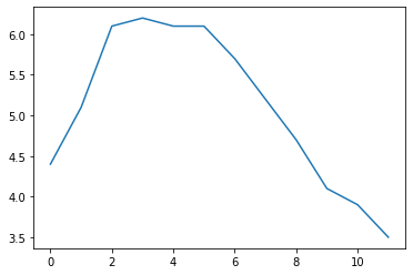

There are many options for plotting your data. It is not necessary to list them all here: if you need a particular type of plot (histograms, pie charts, etc.), just look for it in the excellent Visualization section of pandas’ documentation, and look at the example code.

Handling time

Many datasets have timestamps, and pandas is awesome at manipulating such data: * it can represent periods (such as 2016Q3) and frequencies (such as “monthly”), * it can convert periods to actual timestamps, and vice versa, * it can resample data and aggregate values any way you like, * it can handle timezones.

Time range

Let’s start by creating a time series using pd.date_range(). This returns a DatetimeIndex containing one datetime per hour for 12 hours starting on October 29th 2016 at 5:30pm.

Code

dates = pd.date_range('2016/10/29 5:30pm', periods=12, freq='H')
dates

DatetimeIndex(['2016-10-29 17:30:00', '2016-10-29 18:30:00',
               '2016-10-29 19:30:00', '2016-10-29 20:30:00',
               '2016-10-29 21:30:00', '2016-10-29 22:30:00',
               '2016-10-29 23:30:00', '2016-10-30 00:30:00',
               '2016-10-30 01:30:00', '2016-10-30 02:30:00',
               '2016-10-30 03:30:00', '2016-10-30 04:30:00'],
              dtype='datetime64[ns]', freq='H')

This DatetimeIndex may be used as an index in a Series:

Code

temp_series = pd.Series(temperatures, dates)
temp_series

2016-10-29 17:30:00    4.4
2016-10-29 18:30:00    5.1
2016-10-29 19:30:00    6.1
2016-10-29 20:30:00    6.2
2016-10-29 21:30:00    6.1
2016-10-29 22:30:00    6.1
2016-10-29 23:30:00    5.7
2016-10-30 00:30:00    5.2
2016-10-30 01:30:00    4.7
2016-10-30 02:30:00    4.1
2016-10-30 03:30:00    3.9
2016-10-30 04:30:00    3.5
Freq: H, dtype: float64

Let’s plot this series:

Code

temp_series.plot(kind="bar")

plt.grid(True)
plt.show()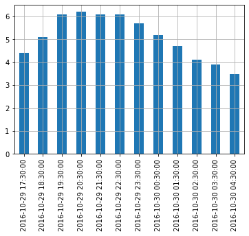

Resampling

Pandas lets us resample a time series very simply. Just call the resample() method and specify a new frequency:

Code

temp_series_freq_2H = temp_series.resample("2H")
temp_series_freq_2H

<pandas.core.resample.DatetimeIndexResampler object at 0x7f69a91f0190>

The resampling operation is actually a deferred operation, which is why we did not get a Series object, but a DatetimeIndexResampler object instead. To actually perform the resampling operation, we can simply call the mean() method: Pandas will compute the mean of every pair of consecutive hours:

Code

temp_series_freq_2H = temp_series_freq_2H.mean()

Let’s plot the result:

Code

temp_series_freq_2H.plot(kind="bar")
plt.show()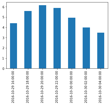

Note how the values have automatically been aggregated into 2-hour periods. If we look at the 6-8pm period, for example, we had a value of 5.1 at 6:30pm, and 6.1 at 7:30pm. After resampling, we just have one value of 5.6, which is the mean of 5.1 and 6.1. Rather than computing the mean, we could have used any other aggregation function, for example we can decide to keep the minimum value of each period:

Code

temp_series_freq_2H = temp_series.resample("2H").min()
temp_series_freq_2H

2016-10-29 16:00:00    4.4
2016-10-29 18:00:00    5.1
2016-10-29 20:00:00    6.1
2016-10-29 22:00:00    5.7
2016-10-30 00:00:00    4.7
2016-10-30 02:00:00    3.9
2016-10-30 04:00:00    3.5
Freq: 2H, dtype: float64

Or, equivalently, we could use the apply() method instead:

Code

temp_series_freq_2H = temp_series.resample("2H").apply(np.min)
temp_series_freq_2H

2016-10-29 16:00:00    4.4
2016-10-29 18:00:00    5.1
2016-10-29 20:00:00    6.1
2016-10-29 22:00:00    5.7
2016-10-30 00:00:00    4.7
2016-10-30 02:00:00    3.9
2016-10-30 04:00:00    3.5
Freq: 2H, dtype: float64

Upsampling and interpolation

This was an example of downsampling. We can also upsample (ie. increase the frequency), but this creates holes in our data:

Code

temp_series_freq_15min = temp_series.resample("15Min").mean()
temp_series_freq_15min.head(n=10) # `head` displays the top n values

2016-10-29 17:30:00    4.4
2016-10-29 17:45:00    NaN
2016-10-29 18:00:00    NaN
2016-10-29 18:15:00    NaN
2016-10-29 18:30:00    5.1
2016-10-29 18:45:00    NaN
2016-10-29 19:00:00    NaN
2016-10-29 19:15:00    NaN
2016-10-29 19:30:00    6.1
2016-10-29 19:45:00    NaN
Freq: 15T, dtype: float64

One solution is to fill the gaps by interpolating. We just call the interpolate() method. The default is to use linear interpolation, but we can also select another method, such as cubic interpolation:

Code

temp_series_freq_15min = temp_series.resample("15Min").interpolate(method="cubic")
temp_series_freq_15min.head(n=10)

2016-10-29 17:30:00    4.400000
2016-10-29 17:45:00    4.452911
2016-10-29 18:00:00    4.605113
2016-10-29 18:15:00    4.829758
2016-10-29 18:30:00    5.100000
2016-10-29 18:45:00    5.388992
2016-10-29 19:00:00    5.669887
2016-10-29 19:15:00    5.915839
2016-10-29 19:30:00    6.100000
2016-10-29 19:45:00    6.203621
Freq: 15T, dtype: float64

Code

temp_series.plot(label="Period: 1 hour")
temp_series_freq_15min.plot(label="Period: 15 minutes")
plt.legend()
plt.show()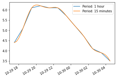

Timezones

By default datetimes are naive: they are not aware of timezones, so 2016-10-30 02:30 might mean October 30th 2016 at 2:30am in Paris or in New York. We can make datetimes timezone aware by calling the tz_localize() method:

Code

temp_series_ny = temp_series.tz_localize("America/New_York")
temp_series_ny

2016-10-29 17:30:00-04:00    4.4
2016-10-29 18:30:00-04:00    5.1
2016-10-29 19:30:00-04:00    6.1
2016-10-29 20:30:00-04:00    6.2
2016-10-29 21:30:00-04:00    6.1
2016-10-29 22:30:00-04:00    6.1
2016-10-29 23:30:00-04:00    5.7
2016-10-30 00:30:00-04:00    5.2
2016-10-30 01:30:00-04:00    4.7
2016-10-30 02:30:00-04:00    4.1
2016-10-30 03:30:00-04:00    3.9
2016-10-30 04:30:00-04:00    3.5
dtype: float64

Note that -04:00 is now appended to all the datetimes. This means that these datetimes refer to UTC - 4 hours.

We can convert these datetimes to Paris time like this:

Code

temp_series_paris = temp_series_ny.tz_convert("Europe/Paris")
temp_series_paris

2016-10-29 23:30:00+02:00    4.4
2016-10-30 00:30:00+02:00    5.1
2016-10-30 01:30:00+02:00    6.1
2016-10-30 02:30:00+02:00    6.2
2016-10-30 02:30:00+01:00    6.1
2016-10-30 03:30:00+01:00    6.1
2016-10-30 04:30:00+01:00    5.7
2016-10-30 05:30:00+01:00    5.2
2016-10-30 06:30:00+01:00    4.7
2016-10-30 07:30:00+01:00    4.1
2016-10-30 08:30:00+01:00    3.9
2016-10-30 09:30:00+01:00    3.5
dtype: float64

You may have noticed that the UTC offset changes from +02:00 to +01:00: this is because France switches to winter time at 3am that particular night (time goes back to 2am). Notice that 2:30am occurs twice! Let’s go back to a naive representation (if you log some data hourly using local time, without storing the timezone, you might get something like this):

Code

temp_series_paris_naive = temp_series_paris.tz_localize(None)
temp_series_paris_naive

2016-10-29 23:30:00    4.4
2016-10-30 00:30:00    5.1
2016-10-30 01:30:00    6.1
2016-10-30 02:30:00    6.2
2016-10-30 02:30:00    6.1
2016-10-30 03:30:00    6.1
2016-10-30 04:30:00    5.7
2016-10-30 05:30:00    5.2
2016-10-30 06:30:00    4.7
2016-10-30 07:30:00    4.1
2016-10-30 08:30:00    3.9
2016-10-30 09:30:00    3.5
dtype: float64

Now 02:30 is really ambiguous. If we try to localize these naive datetimes to the Paris timezone, we get an error:

Code

try:
    temp_series_paris_naive.tz_localize("Europe/Paris")
except Exception as e:
    print(type(e))
    print(e)

<class 'pytz.exceptions.AmbiguousTimeError'>
Cannot infer dst time from 2016-10-30 02:30:00, try using the 'ambiguous' argument

Fortunately using the ambiguous argument we can tell pandas to infer the right DST (Daylight Saving Time) based on the order of the ambiguous timestamps:

Code

temp_series_paris_naive.tz_localize("Europe/Paris", ambiguous="infer")

2016-10-29 23:30:00+02:00    4.4
2016-10-30 00:30:00+02:00    5.1
2016-10-30 01:30:00+02:00    6.1
2016-10-30 02:30:00+02:00    6.2
2016-10-30 02:30:00+01:00    6.1
2016-10-30 03:30:00+01:00    6.1
2016-10-30 04:30:00+01:00    5.7
2016-10-30 05:30:00+01:00    5.2
2016-10-30 06:30:00+01:00    4.7
2016-10-30 07:30:00+01:00    4.1
2016-10-30 08:30:00+01:00    3.9
2016-10-30 09:30:00+01:00    3.5
dtype: float64

Periods

The pd.period_range() function returns a PeriodIndex instead of a DatetimeIndex. For example, let’s get all quarters in 2016 and 2017:

Code

quarters = pd.period_range('2016Q1', periods=8, freq='Q')
quarters

PeriodIndex(['2016Q1', '2016Q2', '2016Q3', '2016Q4', '2017Q1', '2017Q2',
             '2017Q3', '2017Q4'],
            dtype='period[Q-DEC]')

Adding a number N to a PeriodIndex shifts the periods by N times the PeriodIndex’s frequency:

Code

quarters + 3

PeriodIndex(['2016Q4', '2017Q1', '2017Q2', '2017Q3', '2017Q4', '2018Q1',
             '2018Q2', '2018Q3'],
            dtype='period[Q-DEC]')

The asfreq() method lets us change the frequency of the PeriodIndex. All periods are lengthened or shortened accordingly. For example, let’s convert all the quarterly periods to monthly periods (zooming in):

Code

quarters.asfreq("M")

PeriodIndex(['2016-03', '2016-06', '2016-09', '2016-12', '2017-03', '2017-06',
             '2017-09', '2017-12'],
            dtype='period[M]')

By default, the asfreq zooms on the end of each period. We can tell it to zoom on the start of each period instead:

Code

quarters.asfreq("M", how="start")

PeriodIndex(['2016-01', '2016-04', '2016-07', '2016-10', '2017-01', '2017-04',
             '2017-07', '2017-10'],
            dtype='period[M]')

And we can zoom out:

Code

quarters.asfreq("A")

PeriodIndex(['2016', '2016', '2016', '2016', '2017', '2017', '2017', '2017'], dtype='period[A-DEC]')

Of course we can create a Series with a PeriodIndex:

Code

quarterly_revenue = pd.Series([300, 320, 290, 390, 320, 360, 310, 410], index = quarters)
quarterly_revenue

2016Q1    300
2016Q2    320
2016Q3    290
2016Q4    390
2017Q1    320
2017Q2    360
2017Q3    310
2017Q4    410
Freq: Q-DEC, dtype: int64

Code

quarterly_revenue.plot(kind="line")
plt.show()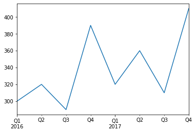

We can convert periods to timestamps by calling to_timestamp. By default this will give us the first day of each period, but by setting how and freq, we can get the last hour of each period:

Code

last_hours = quarterly_revenue.to_timestamp(how="end", freq="H")
last_hours

2016-03-31 23:59:59.999999999    300
2016-06-30 23:59:59.999999999    320
2016-09-30 23:59:59.999999999    290
2016-12-31 23:59:59.999999999    390
2017-03-31 23:59:59.999999999    320
2017-06-30 23:59:59.999999999    360
2017-09-30 23:59:59.999999999    310
2017-12-31 23:59:59.999999999    410
dtype: int64

And back to periods by calling to_period:

Code

last_hours.to_period()

2016Q1    300
2016Q2    320
2016Q3    290
2016Q4    390
2017Q1    320
2017Q2    360
2017Q3    310
2017Q4    410
Freq: Q-DEC, dtype: int64

Pandas also provides many other time-related functions that we recommend you check out in the documentation. To whet your appetite, here is one way to get the last business day of each month in 2016, at 9am:

Code

months_2016 = pd.period_range("2016", periods=12, freq="M")
one_day_after_last_days = months_2016.asfreq("D") + 1
last_bdays = one_day_after_last_days.to_timestamp() - pd.tseries.offsets.BDay()
last_bdays.to_period("H") + 9

PeriodIndex(['2016-01-29 09:00', '2016-02-29 09:00', '2016-03-31 09:00',
             '2016-04-29 09:00', '2016-05-31 09:00', '2016-06-30 09:00',
             '2016-07-29 09:00', '2016-08-31 09:00', '2016-09-30 09:00',
             '2016-10-31 09:00', '2016-11-30 09:00', '2016-12-30 09:00'],
            dtype='period[H]')

DataFrame objects

A DataFrame object represents a spreadsheet, with cell values, column names and row index labels. You can define expressions to compute columns based on other columns, create pivot-tables, group rows, draw graphs, etc. You can see DataFrames as dictionaries of Series.

Creating a DataFrame

You can create a DataFrame by passing a dictionary of Series objects:

Code

people_dict = {
    "weight": pd.Series([68, 83, 112], index=["alice", "bob", "charles"]),
    "birthyear": pd.Series([1984, 1985, 1992], index=["bob", "alice", "charles"], name="year"),
    "children": pd.Series([0, 3], index=["charles", "bob"]),
    "hobby": pd.Series(["Biking", "Dancing"], index=["alice", "bob"]),
}
people = pd.DataFrame(people_dict)
people

	weight	birthyear	children	hobby
alice	68	1985	NaN	Biking
bob	83	1984	3.0	Dancing
charles	112	1992	0.0	NaN

A few things to note: * the Series were automatically aligned based on their index, * missing values are represented as NaN, * Series names are ignored (the name "year" was dropped), * DataFrames are displayed nicely in Jupyter notebooks, woohoo!

You can access columns pretty much as you would expect. They are returned as Series objects:

Code

people["birthyear"]

alice      1985
bob        1984
charles    1992
Name: birthyear, dtype: int64

You can also get multiple columns at once:

Code

people[["birthyear", "hobby"]]

	birthyear	hobby
alice	1985	Biking
bob	1984	Dancing
charles	1992	NaN

If you pass a list of columns and/or index row labels to the DataFrame constructor, it will guarantee that these columns and/or rows will exist, in that order, and no other column/row will exist. For example:

Code

d2 = pd.DataFrame(
        people_dict,
        columns=["birthyear", "weight", "height"],
        index=["bob", "alice", "eugene"]
     )
d2

	birthyear	weight	height
bob	1984.0	83.0	NaN
alice	1985.0	68.0	NaN
eugene	NaN	NaN	NaN

Another convenient way to create a DataFrame is to pass all the values to the constructor as an ndarray, or a list of lists, and specify the column names and row index labels separately:

Code

values = [
            [1985, np.nan, "Biking",   68],
            [1984, 3,      "Dancing",  83],
            [1992, 0,      np.nan,    112]
         ]
d3 = pd.DataFrame(
        values,
        columns=["birthyear", "children", "hobby", "weight"],
        index=["alice", "bob", "charles"]
     )
d3

	birthyear	children	hobby	weight
alice	1985	NaN	Biking	68
bob	1984	3.0	Dancing	83
charles	1992	0.0	NaN	112

To specify missing values, you can either use np.nan or NumPy’s masked arrays:

Code

masked_array = np.ma.asarray(values, dtype=np.object)
masked_array[(0, 2), (1, 2)] = np.ma.masked
d3 = pd.DataFrame(
        masked_array,
        columns=["birthyear", "children", "hobby", "weight"],
        index=["alice", "bob", "charles"]
     )
d3

/opt/conda/lib/python3.7/site-packages/ipykernel_launcher.py:1: DeprecationWarning: `np.object` is a deprecated alias for the builtin `object`. To silence this warning, use `object` by itself. Doing this will not modify any behavior and is safe. 
Deprecated in NumPy 1.20; for more details and guidance: https://numpy.org/devdocs/release/1.20.0-notes.html#deprecations
  """Entry point for launching an IPython kernel.

	birthyear	children	hobby	weight
alice	1985	NaN	Biking	68
bob	1984	3	Dancing	83
charles	1992	0	NaN	112

Instead of an ndarray, you can also pass a DataFrame object:

Code

d4 = pd.DataFrame(
         d3,
         columns=["hobby", "children"],
         index=["alice", "bob"]
     )
d4

	hobby	children
alice	Biking	NaN
bob	Dancing	3

It is also possible to create a DataFrame with a dictionary (or list) of dictionaries (or list):

Code

people = pd.DataFrame({
    "birthyear": {"alice":1985, "bob": 1984, "charles": 1992},
    "hobby": {"alice":"Biking", "bob": "Dancing"},
    "weight": {"alice":68, "bob": 83, "charles": 112},
    "children": {"bob": 3, "charles": 0}
})
people

	birthyear	hobby	weight	children
alice	1985	Biking	68	NaN
bob	1984	Dancing	83	3.0
charles	1992	NaN	112	0.0

Multi-indexing

If all columns are tuples of the same size, then they are understood as a multi-index. The same goes for row index labels. For example:

Code

d5 = pd.DataFrame(
  {
    ("public", "birthyear"):
        {("Paris","alice"):1985, ("Paris","bob"): 1984, ("London","charles"): 1992},
    ("public", "hobby"):
        {("Paris","alice"):"Biking", ("Paris","bob"): "Dancing"},
    ("private", "weight"):
        {("Paris","alice"):68, ("Paris","bob"): 83, ("London","charles"): 112},
    ("private", "children"):
        {("Paris", "alice"):np.nan, ("Paris","bob"): 3, ("London","charles"): 0}
  }
)
d5

		public		private
		birthyear	hobby	weight	children
Paris	alice	1985	Biking	68	NaN
	bob	1984	Dancing	83	3.0
London	charles	1992	NaN	112	0.0

You can now get a DataFrame containing all the "public" columns very simply:

Code

d5["public"]

		birthyear	hobby
Paris	alice	1985	Biking
	bob	1984	Dancing
London	charles	1992	NaN

Code

d5["public", "hobby"]  # Same result as d5["public"]["hobby"]

Paris   alice       Biking
        bob        Dancing
London  charles        NaN
Name: (public, hobby), dtype: object

Dropping a level

Let’s look at d5 again:

Code

d5

		public		private
		birthyear	hobby	weight	children
Paris	alice	1985	Biking	68	NaN
	bob	1984	Dancing	83	3.0
London	charles	1992	NaN	112	0.0

There are two levels of columns, and two levels of indices. We can drop a column level by calling droplevel() (the same goes for indices):

Code

d5.columns = d5.columns.droplevel(level = 0)
d5

		birthyear	hobby	weight	children
Paris	alice	1985	Biking	68	NaN
	bob	1984	Dancing	83	3.0
London	charles	1992	NaN	112	0.0

Transposing

You can swap columns and indices using the T attribute:

Code

d6 = d5.T
d6

	Paris		London
	alice	bob	charles
birthyear	1985	1984	1992
hobby	Biking	Dancing	NaN
weight	68	83	112
children	NaN	3.0	0.0

Stacking and unstacking levels

Calling the stack() method will push the lowest column level after the lowest index:

Code

d7 = d6.stack()
d7

		London	Paris
birthyear	alice	NaN	1985
	bob	NaN	1984
	charles	1992	NaN
hobby	alice	NaN	Biking
	bob	NaN	Dancing
weight	alice	NaN	68
	bob	NaN	83
	charles	112	NaN
children	bob	NaN	3.0
	charles	0.0	NaN

Note that many NaN values appeared. This makes sense because many new combinations did not exist before (eg. there was no bob in London).

Calling unstack() will do the reverse, once again creating many NaN values.

Code

d8 = d7.unstack()
d8

	London			Paris
	alice	bob	charles	alice	bob	charles
birthyear	NaN	NaN	1992	1985	1984	NaN
children	NaN	NaN	0.0	NaN	3.0	NaN
hobby	NaN	NaN	NaN	Biking	Dancing	NaN
weight	NaN	NaN	112	68	83	NaN

If we call unstack again, we end up with a Series object:

Code

d9 = d8.unstack()
d9

London  alice    birthyear        NaN
                 children         NaN
                 hobby            NaN
                 weight           NaN
        bob      birthyear        NaN
                 children         NaN
                 hobby            NaN
                 weight           NaN
        charles  birthyear       1992
                 children         0.0
                 hobby            NaN
                 weight           112
Paris   alice    birthyear       1985
                 children         NaN
                 hobby         Biking
                 weight            68
        bob      birthyear       1984
                 children         3.0
                 hobby        Dancing
                 weight            83
        charles  birthyear        NaN
                 children         NaN
                 hobby            NaN
                 weight           NaN
dtype: object

The stack() and unstack() methods let you select the level to stack/unstack. You can even stack/unstack multiple levels at once:

Code

d10 = d9.unstack(level = (0,1))
d10

	London			Paris
	alice	bob	charles	alice	bob	charles
birthyear	NaN	NaN	1992	1985	1984	NaN
children	NaN	NaN	0.0	NaN	3.0	NaN
hobby	NaN	NaN	NaN	Biking	Dancing	NaN
weight	NaN	NaN	112	68	83	NaN

Most methods return modified copies

As you may have noticed, the stack() and unstack() methods do not modify the object they apply to. Instead, they work on a copy and return that copy. This is true of most methods in pandas.

Accessing rows

Let’s go back to the people DataFrame:

Code

people

	birthyear	hobby	weight	children
alice	1985	Biking	68	NaN
bob	1984	Dancing	83	3.0
charles	1992	NaN	112	0.0

The loc attribute lets you access rows instead of columns. The result is a Series object in which the DataFrame’s column names are mapped to row index labels:

Code

people.loc["charles"]

birthyear    1992
hobby         NaN
weight        112
children      0.0
Name: charles, dtype: object

You can also access rows by integer location using the iloc attribute:

Code

people.iloc[2]

birthyear    1992
hobby         NaN
weight        112
children      0.0
Name: charles, dtype: object

You can also get a slice of rows, and this returns a DataFrame object:

Code

people.iloc[1:3]

	birthyear	hobby	weight	children
bob	1984	Dancing	83	3.0
charles	1992	NaN	112	0.0

Finally, you can pass a boolean array to get the matching rows:

Code

people[np.array([True, False, True])]

	birthyear	hobby	weight	children
alice	1985	Biking	68	NaN
charles	1992	NaN	112	0.0

This is most useful when combined with boolean expressions:

Code

people[people["birthyear"] < 1990]

	birthyear	hobby	weight	children
alice	1985	Biking	68	NaN
bob	1984	Dancing	83	3.0

Adding and removing columns

You can generally treat DataFrame objects like dictionaries of Series, so the following work fine:

Code

people

	birthyear	hobby	weight	children
alice	1985	Biking	68	NaN
bob	1984	Dancing	83	3.0
charles	1992	NaN	112	0.0

Code

people["age"] = 2018 - people["birthyear"]  # adds a new column "age"
people["over 30"] = people["age"] > 30      # adds another column "over 30"
birthyears = people.pop("birthyear")
del people["children"]

people

	hobby	weight	age	over 30
alice	Biking	68	33	True
bob	Dancing	83	34	True
charles	NaN	112	26	False

Code

birthyears

alice      1985
bob        1984
charles    1992
Name: birthyear, dtype: int64

When you add a new colum, it must have the same number of rows. Missing rows are filled with NaN, and extra rows are ignored:

Code

people["pets"] = pd.Series({"bob": 0, "charles": 5, "eugene":1})  # alice is missing, eugene is ignored
people

	hobby	weight	age	over 30	pets
alice	Biking	68	33	True	NaN
bob	Dancing	83	34	True	0.0
charles	NaN	112	26	False	5.0

When adding a new column, it is added at the end (on the right) by default. You can also insert a column anywhere else using the insert() method:

Code

people.insert(1, "height", [172, 181, 185])
people

	hobby	height	weight	age	over 30	pets
alice	Biking	172	68	33	True	NaN
bob	Dancing	181	83	34	True	0.0
charles	NaN	185	112	26	False	5.0

Assigning new columns

You can also create new columns by calling the assign() method. Note that this returns a new DataFrame object, the original is not modified:

Code

people.assign(
    body_mass_index = people["weight"] / (people["height"] / 100) ** 2,
    has_pets = people["pets"] > 0
)

	hobby	height	weight	age	over 30	pets	body_mass_index	has_pets
alice	Biking	172	68	33	True	NaN	22.985398	False
bob	Dancing	181	83	34	True	0.0	25.335002	False
charles	NaN	185	112	26	False	5.0	32.724617	True

Note that you cannot access columns created within the same assignment:

Code

try:
    people.assign(
        body_mass_index = people["weight"] / (people["height"] / 100) ** 2,
        overweight = people["body_mass_index"] > 25
    )
except KeyError as e:
    print("Key error:", e)

Key error: 'body_mass_index'

The solution is to split this assignment in two consecutive assignments:

Code

d6 = people.assign(body_mass_index = people["weight"] / (people["height"] / 100) ** 2)
d6.assign(overweight = d6["body_mass_index"] > 25)

	hobby	height	weight	age	over 30	pets	body_mass_index	overweight
alice	Biking	172	68	33	True	NaN	22.985398	False
bob	Dancing	181	83	34	True	0.0	25.335002	True
charles	NaN	185	112	26	False	5.0	32.724617	True

Having to create a temporary variable d6 is not very convenient. You may want to just chain the assigment calls, but it does not work because the people object is not actually modified by the first assignment:

Code

try:
    (people
         .assign(body_mass_index = people["weight"] / (people["height"] / 100) ** 2)
         .assign(overweight = people["body_mass_index"] > 25)
    )
except KeyError as e:
    print("Key error:", e)

Key error: 'body_mass_index'

But fear not, there is a simple solution. You can pass a function to the assign() method (typically a lambda function), and this function will be called with the DataFrame as a parameter:

Code

(people
     .assign(body_mass_index = lambda df: df["weight"] / (df["height"] / 100) ** 2)
     .assign(overweight = lambda df: df["body_mass_index"] > 25)
)

	hobby	height	weight	age	over 30	pets	body_mass_index	overweight
alice	Biking	172	68	33	True	NaN	22.985398	False
bob	Dancing	181	83	34	True	0.0	25.335002	True
charles	NaN	185	112	26	False	5.0	32.724617	True

Problem solved!

Evaluating an expression

A great feature supported by pandas is expression evaluation. This relies on the numexpr library which must be installed.

Code

people.eval("weight / (height/100) ** 2 > 25")

alice      False
bob         True
charles     True
dtype: bool

Assignment expressions are also supported. Let’s set inplace=True to directly modify the DataFrame rather than getting a modified copy:

Code

people.eval("body_mass_index = weight / (height/100) ** 2", inplace=True)
people

	hobby	height	weight	age	over 30	pets	body_mass_index
alice	Biking	172	68	33	True	NaN	22.985398
bob	Dancing	181	83	34	True	0.0	25.335002
charles	NaN	185	112	26	False	5.0	32.724617

You can use a local or global variable in an expression by prefixing it with '@':

Code

overweight_threshold = 30
people.eval("overweight = body_mass_index > @overweight_threshold", inplace=True)
people

	hobby	height	weight	age	over 30	pets	body_mass_index	overweight
alice	Biking	172	68	33	True	NaN	22.985398	False
bob	Dancing	181	83	34	True	0.0	25.335002	False
charles	NaN	185	112	26	False	5.0	32.724617	True

Querying a DataFrame

The query() method lets you filter a DataFrame based on a query expression:

Code

people.query("age > 30 and pets == 0")

	hobby	height	weight	age	over 30	pets	body_mass_index	overweight
bob	Dancing	181	83	34	True	0.0	25.335002	False

Sorting a DataFrame

You can sort a DataFrame by calling its sort_index method. By default it sorts the rows by their index label, in ascending order, but let’s reverse the order:

Code

people.sort_index(ascending=False)

	hobby	height	weight	age	over 30	pets	body_mass_index	overweight
charles	NaN	185	112	26	False	5.0	32.724617	True
bob	Dancing	181	83	34	True	0.0	25.335002	False
alice	Biking	172	68	33	True	NaN	22.985398	False

Note that sort_index returned a sorted copy of the DataFrame. To modify people directly, we can set the inplace argument to True. Also, we can sort the columns instead of the rows by setting axis=1:

Code

people.sort_index(axis=1, inplace=True)
people

	age	body_mass_index	height	hobby	over 30	overweight	pets	weight
alice	33	22.985398	172	Biking	True	False	NaN	68
bob	34	25.335002	181	Dancing	True	False	0.0	83
charles	26	32.724617	185	NaN	False	True	5.0	112

To sort the DataFrame by the values instead of the labels, we can use sort_values and specify the column to sort by:

Code

people.sort_values(by="age", inplace=True)
people

	age	body_mass_index	height	hobby	over 30	overweight	pets	weight
charles	26	32.724617	185	NaN	False	True	5.0	112
alice	33	22.985398	172	Biking	True	False	NaN	68
bob	34	25.335002	181	Dancing	True	False	0.0	83

Plotting a DataFrame

Just like for Series, pandas makes it easy to draw nice graphs based on a DataFrame.

For example, it is trivial to create a line plot from a DataFrame’s data by calling its plot method:

Code

people.plot(kind = "line", x = "body_mass_index", y = ["height", "weight"])
plt.show()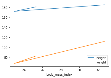

You can pass extra arguments supported by matplotlib’s functions. For example, we can create scatterplot and pass it a list of sizes using the s argument of matplotlib’s scatter() function:

Code

people.plot(kind = "scatter", x = "height", y = "weight", s=[40, 120, 200])
plt.show()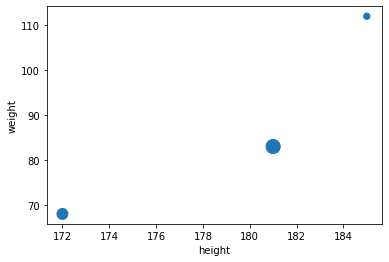

Again, there are way too many options to list here: the best option is to scroll through the Visualization page in pandas’ documentation, find the plot you are interested in and look at the example code.

Operations on DataFrames

Although DataFrames do not try to mimick NumPy arrays, there are a few similarities. Let’s create a DataFrame to demonstrate this:

Code

grades_array = np.array([[8,8,9],[10,9,9],[4, 8, 2], [9, 10, 10]])
grades = pd.DataFrame(grades_array, columns=["sep", "oct", "nov"], index=["alice","bob","charles","darwin"])
grades

	sep	oct	nov
alice	8	8	9
bob	10	9	9
charles	4	8	2
darwin	9	10	10

You can apply NumPy mathematical functions on a DataFrame: the function is applied to all values:

Code

np.sqrt(grades)

	sep	oct	nov
alice	2.828427	2.828427	3.000000
bob	3.162278	3.000000	3.000000
charles	2.000000	2.828427	1.414214
darwin	3.000000	3.162278	3.162278

Similarly, adding a single value to a DataFrame will add that value to all elements in the DataFrame. This is called broadcasting:

Code

grades + 1

	sep	oct	nov
alice	9	9	10
bob	11	10	10
charles	5	9	3
darwin	10	11	11

Of course, the same is true for all other binary operations, including arithmetic (*,/,**…) and conditional (>, ==…) operations:

Code

grades >= 5

	sep	oct	nov
alice	True	True	True
bob	True	True	True
charles	False	True	False
darwin	True	True	True

Aggregation operations, such as computing the max, the sum or the mean of a DataFrame, apply to each column, and you get back a Series object:

Code

grades.mean()

sep    7.75
oct    8.75
nov    7.50
dtype: float64

The all method is also an aggregation operation: it checks whether all values are True or not. Let’s see during which months all students got a grade greater than 5:

Code

(grades > 5).all()

sep    False
oct     True
nov    False
dtype: bool

Most of these functions take an optional axis parameter which lets you specify along which axis of the DataFrame you want the operation executed. The default is axis=0, meaning that the operation is executed vertically (on each column). You can set axis=1 to execute the operation horizontally (on each row). For example, let’s find out which students had all grades greater than 5:

Code

(grades > 5).all(axis = 1)

alice       True
bob         True
charles    False
darwin      True
dtype: bool

The any method returns True if any value is True. Let’s see who got at least one grade 10:

Code

(grades == 10).any(axis = 1)

alice      False
bob         True
charles    False
darwin      True
dtype: bool

If you add a Series object to a DataFrame (or execute any other binary operation), pandas attempts to broadcast the operation to all rows in the DataFrame. This only works if the Series has the same size as the DataFrames rows. For example, let’s subtract the mean of the DataFrame (a Series object) from the DataFrame:

Code

grades - grades.mean()  # equivalent to: grades - [7.75, 8.75, 7.50]

	sep	oct	nov
alice	0.25	-0.75	1.5
bob	2.25	0.25	1.5
charles	-3.75	-0.75	-5.5
darwin	1.25	1.25	2.5

We subtracted 7.75 from all September grades, 8.75 from October grades and 7.50 from November grades. It is equivalent to subtracting this DataFrame:

Code

pd.DataFrame([[7.75, 8.75, 7.50]]*4, index=grades.index, columns=grades.columns)

	sep	oct	nov
alice	7.75	8.75	7.5
bob	7.75	8.75	7.5
charles	7.75	8.75	7.5
darwin	7.75	8.75	7.5

If you want to subtract the global mean from every grade, here is one way to do it:

Code

grades - grades.values.mean() # subtracts the global mean (8.00) from all grades

	sep	oct	nov
alice	0.0	0.0	1.0
bob	2.0	1.0	1.0
charles	-4.0	0.0	-6.0
darwin	1.0	2.0	2.0

Automatic alignment

Similar to Series, when operating on multiple DataFrames, pandas automatically aligns them by row index label, but also by column names. Let’s create a DataFrame with bonus points for each person from October to December:

Code

bonus_array = np.array([[0,np.nan,2],[np.nan,1,0],[0, 1, 0], [3, 3, 0]])
bonus_points = pd.DataFrame(bonus_array, columns=["oct", "nov", "dec"], index=["bob","colin", "darwin", "charles"])
bonus_points

	oct	nov	dec
bob	0.0	NaN	2.0
colin	NaN	1.0	0.0
darwin	0.0	1.0	0.0
charles	3.0	3.0	0.0

Code

grades + bonus_points

	dec	nov	oct	sep
alice	NaN	NaN	NaN	NaN
bob	NaN	NaN	9.0	NaN
charles	NaN	5.0	11.0	NaN
colin	NaN	NaN	NaN	NaN
darwin	NaN	11.0	10.0	NaN

Looks like the addition worked in some cases but way too many elements are now empty. That’s because when aligning the DataFrames, some columns and rows were only present on one side, and thus they were considered missing on the other side (NaN). Then adding NaN to a number results in NaN, hence the result.

Handling missing data

Dealing with missing data is a frequent task when working with real life data. Pandas offers a few tools to handle missing data.

Let’s try to fix the problem above. For example, we can decide that missing data should result in a zero, instead of NaN. We can replace all NaN values by a any value using the fillna() method:

Code

(grades + bonus_points).fillna(0)

	dec	nov	oct	sep
alice	0.0	0.0	0.0	0.0
bob	0.0	0.0	9.0	0.0
charles	0.0	5.0	11.0	0.0
colin	0.0	0.0	0.0	0.0
darwin	0.0	11.0	10.0	0.0

It’s a bit unfair that we’re setting grades to zero in September, though. Perhaps we should decide that missing grades are missing grades, but missing bonus points should be replaced by zeros:

Code

fixed_bonus_points = bonus_points.fillna(0)
fixed_bonus_points.insert(0, "sep", 0)
fixed_bonus_points.loc["alice"] = 0
grades + fixed_bonus_points

	dec	nov	oct	sep
alice	NaN	9.0	8.0	8.0
bob	NaN	9.0	9.0	10.0
charles	NaN	5.0	11.0	4.0
colin	NaN	NaN	NaN	NaN
darwin	NaN	11.0	10.0	9.0

That’s much better: although we made up some data, we have not been too unfair.

Another way to handle missing data is to interpolate. Let’s look at the bonus_points DataFrame again:

Code

bonus_points

	oct	nov	dec
bob	0.0	NaN	2.0
colin	NaN	1.0	0.0
darwin	0.0	1.0	0.0
charles	3.0	3.0	0.0

Now let’s call the interpolate method. By default, it interpolates vertically (axis=0), so let’s tell it to interpolate horizontally (axis=1).

Code

bonus_points.interpolate(axis=1)

	oct	nov	dec
bob	0.0	1.0	2.0
colin	NaN	1.0	0.0
darwin	0.0	1.0	0.0
charles	3.0	3.0	0.0

Bob had 0 bonus points in October, and 2 in December. When we interpolate for November, we get the mean: 1 bonus point. Colin had 1 bonus point in November, but we do not know how many bonus points he had in September, so we cannot interpolate, this is why there is still a missing value in October after interpolation. To fix this, we can set the September bonus points to 0 before interpolation.

Code

better_bonus_points = bonus_points.copy()
better_bonus_points.insert(0, "sep", 0)
better_bonus_points.loc["alice"] = 0
better_bonus_points = better_bonus_points.interpolate(axis=1)
better_bonus_points

	sep	oct	nov	dec
bob	0.0	0.0	1.0	2.0
colin	0.0	0.5	1.0	0.0
darwin	0.0	0.0	1.0	0.0
charles	0.0	3.0	3.0	0.0
alice	0.0	0.0	0.0	0.0

Great, now we have reasonable bonus points everywhere. Let’s find out the final grades:

Code

grades + better_bonus_points

	dec	nov	oct	sep
alice	NaN	9.0	8.0	8.0
bob	NaN	10.0	9.0	10.0
charles	NaN	5.0	11.0	4.0
colin	NaN	NaN	NaN	NaN
darwin	NaN	11.0	10.0	9.0

It is slightly annoying that the September column ends up on the right. This is because the DataFrames we are adding do not have the exact same columns (the grades DataFrame is missing the "dec" column), so to make things predictable, pandas orders the final columns alphabetically. To fix this, we can simply add the missing column before adding:

Code

grades["dec"] = np.nan
final_grades = grades + better_bonus_points
final_grades

	sep	oct	nov	dec
alice	8.0	8.0	9.0	NaN
bob	10.0	9.0	10.0	NaN
charles	4.0	11.0	5.0	NaN
colin	NaN	NaN	NaN	NaN
darwin	9.0	10.0	11.0	NaN

There’s not much we can do about December and Colin: it’s bad enough that we are making up bonus points, but we can’t reasonably make up grades (well I guess some teachers probably do). So let’s call the dropna() method to get rid of rows that are full of NaNs:

Code

final_grades_clean = final_grades.dropna(how="all")
final_grades_clean

	sep	oct	nov	dec
alice	8.0	8.0	9.0	NaN
bob	10.0	9.0	10.0	NaN
charles	4.0	11.0	5.0	NaN
darwin	9.0	10.0	11.0	NaN

Now let’s remove columns that are full of NaNs by setting the axis argument to 1:

Code

final_grades_clean = final_grades_clean.dropna(axis=1, how="all")
final_grades_clean

	sep	oct	nov
alice	8.0	8.0	9.0
bob	10.0	9.0	10.0
charles	4.0	11.0	5.0
darwin	9.0	10.0	11.0

Aggregating with groupby

Similar to the SQL language, pandas allows grouping your data into groups to run calculations over each group.

First, let’s add some extra data about each person so we can group them, and let’s go back to the final_grades DataFrame so we can see how NaN values are handled:

Code

final_grades["hobby"] = ["Biking", "Dancing", np.nan, "Dancing", "Biking"]
final_grades

	sep	oct	nov	dec	hobby
alice	8.0	8.0	9.0	NaN	Biking
bob	10.0	9.0	10.0	NaN	Dancing
charles	4.0	11.0	5.0	NaN	NaN
colin	NaN	NaN	NaN	NaN	Dancing
darwin	9.0	10.0	11.0	NaN	Biking

Now let’s group data in this DataFrame by hobby:

Code

grouped_grades = final_grades.groupby("hobby")
grouped_grades

<pandas.core.groupby.generic.DataFrameGroupBy object at 0x7f697dab7310>

We are ready to compute the average grade per hobby:

Code

grouped_grades.mean()

	sep	oct	nov	dec
hobby
Biking	8.5	9.0	10.0	NaN
Dancing	10.0	9.0	10.0	NaN

That was easy! Note that the NaN values have simply been skipped when computing the means.

Pivot tables

Pandas supports spreadsheet-like pivot tables that allow quick data summarization. To illustrate this, let’s create a simple DataFrame:

Code

bonus_points

	oct	nov	dec
bob	0.0	NaN	2.0
colin	NaN	1.0	0.0
darwin	0.0	1.0	0.0
charles	3.0	3.0	0.0

Code

more_grades = final_grades_clean.stack().reset_index()
more_grades.columns = ["name", "month", "grade"]
more_grades["bonus"] = [np.nan, np.nan, np.nan, 0, np.nan, 2, 3, 3, 0, 0, 1, 0]
more_grades

	name	month	grade	bonus
0	alice	sep	8.0	NaN
1	alice	oct	8.0	NaN
2	alice	nov	9.0	NaN
3	bob	sep	10.0	0.0
4	bob	oct	9.0	NaN
5	bob	nov	10.0	2.0
6	charles	sep	4.0	3.0
7	charles	oct	11.0	3.0
8	charles	nov	5.0	0.0
9	darwin	sep	9.0	0.0
10	darwin	oct	10.0	1.0
11	darwin	nov	11.0	0.0

Now we can call the pd.pivot_table() function for this DataFrame, asking to group by the name column. By default, pivot_table() computes the mean of each numeric column:

Code

pd.pivot_table(more_grades, index="name")

	bonus	grade
name
alice	NaN	8.333333
bob	1.000000	9.666667
charles	2.000000	6.666667
darwin	0.333333	10.000000

We can change the aggregation function by setting the aggfunc argument, and we can also specify the list of columns whose values will be aggregated:

Code

pd.pivot_table(more_grades, index="name", values=["grade","bonus"], aggfunc=np.max)

	bonus	grade
name
alice	NaN	9.0
bob	2.0	10.0
charles	3.0	11.0
darwin	1.0	11.0

We can also specify the columns to aggregate over horizontally, and request the grand totals for each row and column by setting margins=True:

Code

pd.pivot_table(more_grades, index="name", values="grade", columns="month", margins=True)

month	nov	oct	sep	All
name
alice	9.00	8.0	8.00	8.333333
bob	10.00	9.0	10.00	9.666667
charles	5.00	11.0	4.00	6.666667
darwin	11.00	10.0	9.00	10.000000
All	8.75	9.5	7.75	8.666667

Finally, we can specify multiple index or column names, and pandas will create multi-level indices:

Code

pd.pivot_table(more_grades, index=("name", "month"), margins=True)

		bonus	grade
name	month
alice	nov	NaN	9.00
	oct	NaN	8.00
	sep	NaN	8.00
bob	nov	2.000	10.00
	oct	NaN	9.00
	sep	0.000	10.00
charles	nov	0.000	5.00
	oct	3.000	11.00
	sep	3.000	4.00
darwin	nov	0.000	11.00
	oct	1.000	10.00
	sep	0.000	9.00
All		1.125	8.75

Overview functions

When dealing with large DataFrames, it is useful to get a quick overview of its content. Pandas offers a few functions for this. First, let’s create a large DataFrame with a mix of numeric values, missing values and text values. Notice how Jupyter displays only the corners of the DataFrame:

Code

much_data = np.fromfunction(lambda x,y: (x+y*y)%17*11, (10000, 26))
large_df = pd.DataFrame(much_data, columns=list("ABCDEFGHIJKLMNOPQRSTUVWXYZ"))
large_df[large_df % 16 == 0] = np.nan
large_df.insert(3,"some_text", "Blabla")
large_df

	A	B	C	some_text	D	E	F	G	H	I	...	Q	R	S	T	U	V	W	X	Y	Z
0	NaN	11.0	44.0	Blabla	99.0	NaN	88.0	22.0	165.0	143.0	...	11.0	NaN	11.0	44.0	99.0	NaN	88.0	22.0	165.0	143.0
1	11.0	22.0	55.0	Blabla	110.0	NaN	99.0	33.0	NaN	154.0	...	22.0	11.0	22.0	55.0	110.0	NaN	99.0	33.0	NaN	154.0
2	22.0	33.0	66.0	Blabla	121.0	11.0	110.0	44.0	NaN	165.0	...	33.0	22.0	33.0	66.0	121.0	11.0	110.0	44.0	NaN	165.0
3	33.0	44.0	77.0	Blabla	132.0	22.0	121.0	55.0	11.0	NaN	...	44.0	33.0	44.0	77.0	132.0	22.0	121.0	55.0	11.0	NaN
4	44.0	55.0	88.0	Blabla	143.0	33.0	132.0	66.0	22.0	NaN	...	55.0	44.0	55.0	88.0	143.0	33.0	132.0	66.0	22.0	NaN
...	...	...	...	...	...	...	...	...	...	...	...	...	...	...	...	...	...	...	...	...	...
9995	NaN	NaN	33.0	Blabla	88.0	165.0	77.0	11.0	154.0	132.0	...	NaN	NaN	NaN	33.0	88.0	165.0	77.0	11.0	154.0	132.0
9996	NaN	11.0	44.0	Blabla	99.0	NaN	88.0	22.0	165.0	143.0	...	11.0	NaN	11.0	44.0	99.0	NaN	88.0	22.0	165.0	143.0
9997	11.0	22.0	55.0	Blabla	110.0	NaN	99.0	33.0	NaN	154.0	...	22.0	11.0	22.0	55.0	110.0	NaN	99.0	33.0	NaN	154.0
9998	22.0	33.0	66.0	Blabla	121.0	11.0	110.0	44.0	NaN	165.0	...	33.0	22.0	33.0	66.0	121.0	11.0	110.0	44.0	NaN	165.0
9999	33.0	44.0	77.0	Blabla	132.0	22.0	121.0	55.0	11.0	NaN	...	44.0	33.0	44.0	77.0	132.0	22.0	121.0	55.0	11.0	NaN

10000 rows × 27 columns

The head() method returns the top 5 rows:

Code

large_df.head()

	A	B	C	some_text	D	E	F	G	H	I	...	Q	R	S	T	U	V	W	X	Y	Z
0	NaN	11.0	44.0	Blabla	99.0	NaN	88.0	22.0	165.0	143.0	...	11.0	NaN	11.0	44.0	99.0	NaN	88.0	22.0	165.0	143.0
1	11.0	22.0	55.0	Blabla	110.0	NaN	99.0	33.0	NaN	154.0	...	22.0	11.0	22.0	55.0	110.0	NaN	99.0	33.0	NaN	154.0
2	22.0	33.0	66.0	Blabla	121.0	11.0	110.0	44.0	NaN	165.0	...	33.0	22.0	33.0	66.0	121.0	11.0	110.0	44.0	NaN	165.0
3	33.0	44.0	77.0	Blabla	132.0	22.0	121.0	55.0	11.0	NaN	...	44.0	33.0	44.0	77.0	132.0	22.0	121.0	55.0	11.0	NaN
4	44.0	55.0	88.0	Blabla	143.0	33.0	132.0	66.0	22.0	NaN	...	55.0	44.0	55.0	88.0	143.0	33.0	132.0	66.0	22.0	NaN

5 rows × 27 columns

Of course there’s also a tail() function to view the bottom 5 rows. You can pass the number of rows you want:

Code

large_df.tail(n=2)

	A	B	C	some_text	D	E	F	G	H	I	...	Q	R	S	T	U	V	W	X	Y	Z
9998	22.0	33.0	66.0	Blabla	121.0	11.0	110.0	44.0	NaN	165.0	...	33.0	22.0	33.0	66.0	121.0	11.0	110.0	44.0	NaN	165.0
9999	33.0	44.0	77.0	Blabla	132.0	22.0	121.0	55.0	11.0	NaN	...	44.0	33.0	44.0	77.0	132.0	22.0	121.0	55.0	11.0	NaN

2 rows × 27 columns

The info() method prints out a summary of each columns contents:

Code

large_df.info()

<class 'pandas.core.frame.DataFrame'>
RangeIndex: 10000 entries, 0 to 9999
Data columns (total 27 columns):
 #   Column     Non-Null Count  Dtype  
---  ------     --------------  -----  
 0   A          8823 non-null   float64
 1   B          8824 non-null   float64
 2   C          8824 non-null   float64
 3   some_text  10000 non-null  object 
 4   D          8824 non-null   float64
 5   E          8822 non-null   float64
 6   F          8824 non-null   float64
 7   G          8824 non-null   float64
 8   H          8822 non-null   float64
 9   I          8823 non-null   float64
 10  J          8823 non-null   float64
 11  K          8822 non-null   float64
 12  L          8824 non-null   float64
 13  M          8824 non-null   float64
 14  N          8822 non-null   float64
 15  O          8824 non-null   float64
 16  P          8824 non-null   float64
 17  Q          8824 non-null   float64
 18  R          8823 non-null   float64
 19  S          8824 non-null   float64
 20  T          8824 non-null   float64
 21  U          8824 non-null   float64
 22  V          8822 non-null   float64
 23  W          8824 non-null   float64
 24  X          8824 non-null   float64
 25  Y          8822 non-null   float64
 26  Z          8823 non-null   float64
dtypes: float64(26), object(1)
memory usage: 2.1+ MB

Finally, the describe() method gives a nice overview of the main aggregated values over each column: * count: number of non-null (not NaN) values * mean: mean of non-null values * std: standard deviation of non-null values * min: minimum of non-null values * 25%, 50%, 75%: 25th, 50th and 75th percentile of non-null values * max: maximum of non-null values

Code

large_df.describe()

	A	B	C	D	E	F	G	H	I	J	...	Q	R	S	T	U	V	W	X	Y	Z
count	8823.000000	8824.000000	8824.000000	8824.000000	8822.000000	8824.000000	8824.000000	8822.000000	8823.000000	8823.000000	...	8824.000000	8823.000000	8824.000000	8824.000000	8824.000000	8822.000000	8824.000000	8824.000000	8822.000000	8823.000000
mean	87.977559	87.972575	87.987534	88.012466	87.983791	88.007480	87.977561	88.000000	88.022441	88.022441	...	87.972575	87.977559	87.972575	87.987534	88.012466	87.983791	88.007480	87.977561	88.000000	88.022441
std	47.535911	47.535523	47.521679	47.521679	47.535001	47.519371	47.529755	47.536879	47.535911	47.535911	...	47.535523	47.535911	47.535523	47.521679	47.521679	47.535001	47.519371	47.529755	47.536879	47.535911
min	11.000000	11.000000	11.000000	11.000000	11.000000	11.000000	11.000000	11.000000	11.000000	11.000000	...	11.000000	11.000000	11.000000	11.000000	11.000000	11.000000	11.000000	11.000000	11.000000	11.000000
25%	44.000000	44.000000	44.000000	44.000000	44.000000	44.000000	44.000000	44.000000	44.000000	44.000000	...	44.000000	44.000000	44.000000	44.000000	44.000000	44.000000	44.000000	44.000000	44.000000	44.000000
50%	88.000000	88.000000	88.000000	88.000000	88.000000	88.000000	88.000000	88.000000	88.000000	88.000000	...	88.000000	88.000000	88.000000	88.000000	88.000000	88.000000	88.000000	88.000000	88.000000	88.000000
75%	132.000000	132.000000	132.000000	132.000000	132.000000	132.000000	132.000000	132.000000	132.000000	132.000000	...	132.000000	132.000000	132.000000	132.000000	132.000000	132.000000	132.000000	132.000000	132.000000	132.000000
max	165.000000	165.000000	165.000000	165.000000	165.000000	165.000000	165.000000	165.000000	165.000000	165.000000	...	165.000000	165.000000	165.000000	165.000000	165.000000	165.000000	165.000000	165.000000	165.000000	165.000000

8 rows × 26 columns

Saving & loading

Pandas can save DataFrames to various backends, including file formats such as CSV, Excel, JSON, HTML and HDF5, or to a SQL database. Let’s create a DataFrame to demonstrate this:

Code

my_df = pd.DataFrame(
    [["Biking", 68.5, 1985, np.nan], ["Dancing", 83.1, 1984, 3]], 
    columns=["hobby","weight","birthyear","children"],
    index=["alice", "bob"]
)
my_df

	hobby	weight	birthyear	children
alice	Biking	68.5	1985	NaN
bob	Dancing	83.1	1984	3.0

Saving

Let’s save it to CSV, HTML and JSON:

Code

my_df.to_csv("my_df.csv")
my_df.to_html("my_df.html")
my_df.to_json("my_df.json")

Done! Let’s take a peek at what was saved:

Code

for filename in ("my_df.csv", "my_df.html", "my_df.json"):
    print("#", filename)
    with open(filename, "rt") as f:
        print(f.read())
        print()

# my_df.csv
,hobby,weight,birthyear,children
alice,Biking,68.5,1985,
bob,Dancing,83.1,1984,3.0


# my_df.html
<table border="1" class="dataframe">
  <thead>
    <tr style="text-align: right;">
      <th></th>
      <th>hobby</th>
      <th>weight</th>
      <th>birthyear</th>
      <th>children</th>
    </tr>
  </thead>
  <tbody>
    <tr>
      <th>alice</th>
      <td>Biking</td>
      <td>68.5</td>
      <td>1985</td>
      <td>NaN</td>
    </tr>
    <tr>
      <th>bob</th>
      <td>Dancing</td>
      <td>83.1</td>
      <td>1984</td>
      <td>3.0</td>
    </tr>
  </tbody>
</table>

# my_df.json
{"hobby":{"alice":"Biking","bob":"Dancing"},"weight":{"alice":68.5,"bob":83.1},"birthyear":{"alice":1985,"bob":1984},"children":{"alice":null,"bob":3.0}}

Note that the index is saved as the first column (with no name) in a CSV file, as <th> tags in HTML and as keys in JSON.

Saving to other formats works very similarly, but some formats require extra libraries to be installed. For example, saving to Excel requires the openpyxl library:

Code

try:
    my_df.to_excel("my_df.xlsx", sheet_name='People')
except ImportError as e:
    print(e)

No module named 'openpyxl'

Loading

Now let’s load our CSV file back into a DataFrame:

Code

my_df_loaded = pd.read_csv("my_df.csv", index_col=0)
my_df_loaded

	hobby	weight	birthyear	children
alice	Biking	68.5	1985	NaN
bob	Dancing	83.1	1984	3.0

As you might guess, there are similar read_json, read_html, read_excel functions as well. We can also read data straight from the Internet. For example, let’s load the top 1,000 U.S. cities from github:

Code

us_cities = None
try:
    csv_url = "https://raw.githubusercontent.com/plotly/datasets/master/us-cities-top-1k.csv"
    us_cities = pd.read_csv(csv_url, index_col=0)
    us_cities = us_cities.head()
except IOError as e:
    print(e)
us_cities

	State	Population	lat	lon
City
Marysville	Washington	63269	48.051764	-122.177082
Perris	California	72326	33.782519	-117.228648
Cleveland	Ohio	390113	41.499320	-81.694361
Worcester	Massachusetts	182544	42.262593	-71.802293
Columbia	South Carolina	133358	34.000710	-81.034814

There are more options available, in particular regarding datetime format. Check out the documentation for more details.

Combining DataFrames

SQL-like joins

One powerful feature of pandas is it’s ability to perform SQL-like joins on DataFrames. Various types of joins are supported: inner joins, left/right outer joins and full joins. To illustrate this, let’s start by creating a couple simple DataFrames:

Code

city_loc = pd.DataFrame(
    [
        ["CA", "San Francisco", 37.781334, -122.416728],
        ["NY", "New York", 40.705649, -74.008344],
        ["FL", "Miami", 25.791100, -80.320733],
        ["OH", "Cleveland", 41.473508, -81.739791],
        ["UT", "Salt Lake City", 40.755851, -111.896657]
    ], columns=["state", "city", "lat", "lng"])
city_loc

	state	city	lat	lng
0	CA	San Francisco	37.781334	-122.416728
1	NY	New York	40.705649	-74.008344
2	FL	Miami	25.791100	-80.320733
3	OH	Cleveland	41.473508	-81.739791
4	UT	Salt Lake City	40.755851	-111.896657

Code

city_pop = pd.DataFrame(
    [
        [808976, "San Francisco", "California"],
        [8363710, "New York", "New-York"],
        [413201, "Miami", "Florida"],
        [2242193, "Houston", "Texas"]
    ], index=[3,4,5,6], columns=["population", "city", "state"])
city_pop

	population	city	state
3	808976	San Francisco	California
4	8363710	New York	New-York
5	413201	Miami	Florida
6	2242193	Houston	Texas

Now let’s join these DataFrames using the merge() function:

Code

pd.merge(left=city_loc, right=city_pop, on="city")

	state_x	city	lat	lng	population	state_y
0	CA	San Francisco	37.781334	-122.416728	808976	California
1	NY	New York	40.705649	-74.008344	8363710	New-York
2	FL	Miami	25.791100	-80.320733	413201	Florida

Note that both DataFrames have a column named state, so in the result they got renamed to state_x and state_y.

Also, note that Cleveland, Salt Lake City and Houston were dropped because they don’t exist in both DataFrames. This is the equivalent of a SQL INNER JOIN. If you want a FULL OUTER JOIN, where no city gets dropped and NaN values are added, you must specify how="outer":

Code

all_cities = pd.merge(left=city_loc, right=city_pop, on="city", how="outer")
all_cities

	state_x	city	lat	lng	population	state_y
0	CA	San Francisco	37.781334	-122.416728	808976.0	California
1	NY	New York	40.705649	-74.008344	8363710.0	New-York
2	FL	Miami	25.791100	-80.320733	413201.0	Florida
3	OH	Cleveland	41.473508	-81.739791	NaN	NaN
4	UT	Salt Lake City	40.755851	-111.896657	NaN	NaN
5	NaN	Houston	NaN	NaN	2242193.0	Texas

Of course LEFT OUTER JOIN is also available by setting how="left": only the cities present in the left DataFrame end up in the result. Similarly, with how="right" only cities in the right DataFrame appear in the result. For example:

Code

pd.merge(left=city_loc, right=city_pop, on="city", how="right")

	state_x	city	lat	lng	population	state_y
0	CA	San Francisco	37.781334	-122.416728	808976	California
1	NY	New York	40.705649	-74.008344	8363710	New-York
2	FL	Miami	25.791100	-80.320733	413201	Florida
3	NaN	Houston	NaN	NaN	2242193	Texas

If the key to join on is actually in one (or both) DataFrame’s index, you must use left_index=True and/or right_index=True. If the key column names differ, you must use left_on and right_on. For example:

Code

city_pop2 = city_pop.copy()
city_pop2.columns = ["population", "name", "state"]
pd.merge(left=city_loc, right=city_pop2, left_on="city", right_on="name")

	state_x	city	lat	lng	population	name	state_y
0	CA	San Francisco	37.781334	-122.416728	808976	San Francisco	California
1	NY	New York	40.705649	-74.008344	8363710	New York	New-York
2	FL	Miami	25.791100	-80.320733	413201	Miami	Florida

Concatenation

Rather than joining DataFrames, we may just want to concatenate them. That’s what concat() is for:

Code

result_concat = pd.concat([city_loc, city_pop])
result_concat

	state	city	lat	lng	population
0	CA	San Francisco	37.781334	-122.416728	NaN
1	NY	New York	40.705649	-74.008344	NaN
2	FL	Miami	25.791100	-80.320733	NaN
3	OH	Cleveland	41.473508	-81.739791	NaN
4	UT	Salt Lake City	40.755851	-111.896657	NaN
3	California	San Francisco	NaN	NaN	808976.0
4	New-York	New York	NaN	NaN	8363710.0
5	Florida	Miami	NaN	NaN	413201.0
6	Texas	Houston	NaN	NaN	2242193.0

Note that this operation aligned the data horizontally (by columns) but not vertically (by rows). In this example, we end up with multiple rows having the same index (eg. 3). Pandas handles this rather gracefully:

Code

result_concat.loc[3]

	state	city	lat	lng	population
3	OH	Cleveland	41.473508	-81.739791	NaN
3	California	San Francisco	NaN	NaN	808976.0

Or you can tell pandas to just ignore the index:

Code

pd.concat([city_loc, city_pop], ignore_index=True)

	state	city	lat	lng	population
0	CA	San Francisco	37.781334	-122.416728	NaN
1	NY	New York	40.705649	-74.008344	NaN
2	FL	Miami	25.791100	-80.320733	NaN
3	OH	Cleveland	41.473508	-81.739791	NaN
4	UT	Salt Lake City	40.755851	-111.896657	NaN
5	California	San Francisco	NaN	NaN	808976.0
6	New-York	New York	NaN	NaN	8363710.0
7	Florida	Miami	NaN	NaN	413201.0
8	Texas	Houston	NaN	NaN	2242193.0

Notice that when a column does not exist in a DataFrame, it acts as if it was filled with NaN values. If we set join="inner", then only columns that exist in both DataFrames are returned:

Code

pd.concat([city_loc, city_pop], join="inner")

	state	city
0	CA	San Francisco
1	NY	New York
2	FL	Miami
3	OH	Cleveland
4	UT	Salt Lake City
3	California	San Francisco
4	New-York	New York
5	Florida	Miami
6	Texas	Houston

You can concatenate DataFrames horizontally instead of vertically by setting axis=1:

Code

pd.concat([city_loc, city_pop], axis=1)

	state	city	lat	lng	population	city	state
0	CA	San Francisco	37.781334	-122.416728	NaN	NaN	NaN
1	NY	New York	40.705649	-74.008344	NaN	NaN	NaN
2	FL	Miami	25.791100	-80.320733	NaN	NaN	NaN
3	OH	Cleveland	41.473508	-81.739791	808976.0	San Francisco	California
4	UT	Salt Lake City	40.755851	-111.896657	8363710.0	New York	New-York
5	NaN	NaN	NaN	NaN	413201.0	Miami	Florida
6	NaN	NaN	NaN	NaN	2242193.0	Houston	Texas

In this case it really does not make much sense because the indices do not align well (eg. Cleveland and San Francisco end up on the same row, because they shared the index label 3). So let’s reindex the DataFrames by city name before concatenating:

Code

pd.concat([city_loc.set_index("city"), city_pop.set_index("city")], axis=1)

	state	lat	lng	population	state
city
San Francisco	CA	37.781334	-122.416728	808976.0	California
New York	NY	40.705649	-74.008344	8363710.0	New-York
Miami	FL	25.791100	-80.320733	413201.0	Florida
Cleveland	OH	41.473508	-81.739791	NaN	NaN
Salt Lake City	UT	40.755851	-111.896657	NaN	NaN
Houston	NaN	NaN	NaN	2242193.0	Texas

This looks a lot like a FULL OUTER JOIN, except that the state columns were not renamed to state_x and state_y, and the city column is now the index.

The append() method is a useful shorthand for concatenating DataFrames vertically:

Code

city_loc.append(city_pop)

	state	city	lat	lng	population
0	CA	San Francisco	37.781334	-122.416728	NaN
1	NY	New York	40.705649	-74.008344	NaN
2	FL	Miami	25.791100	-80.320733	NaN
3	OH	Cleveland	41.473508	-81.739791	NaN
4	UT	Salt Lake City	40.755851	-111.896657	NaN
3	California	San Francisco	NaN	NaN	808976.0
4	New-York	New York	NaN	NaN	8363710.0
5	Florida	Miami	NaN	NaN	413201.0
6	Texas	Houston	NaN	NaN	2242193.0

As always in pandas, the append() method does not actually modify city_loc: it works on a copy and returns the modified copy.

Categories

It is quite frequent to have values that represent categories, for example 1 for female and 2 for male, or "A" for Good, "B" for Average, "C" for Bad. These categorical values can be hard to read and cumbersome to handle, but fortunately pandas makes it easy. To illustrate this, let’s take the city_pop DataFrame we created earlier, and add a column that represents a category:

Code

city_eco = city_pop.copy()
city_eco["eco_code"] = [17, 17, 34, 20]
city_eco

	population	city	state	eco_code
3	808976	San Francisco	California	17
4	8363710	New York	New-York	17
5	413201	Miami	Florida	34
6	2242193	Houston	Texas	20

Right now the eco_code column is full of apparently meaningless codes. Let’s fix that. First, we will create a new categorical column based on the eco_codes:

Code

city_eco["economy"] = city_eco["eco_code"].astype('category')
city_eco["economy"].cat.categories

Int64Index([17, 20, 34], dtype='int64')

Now we can give each category a meaningful name:

Code

city_eco["economy"].cat.categories = ["Finance", "Energy", "Tourism"]
city_eco

	population	city	state	eco_code	economy
3	808976	San Francisco	California	17	Finance
4	8363710	New York	New-York	17	Finance
5	413201	Miami	Florida	34	Tourism
6	2242193	Houston	Texas	20	Energy

Note that categorical values are sorted according to their categorical order, not their alphabetical order:

Code

city_eco.sort_values(by="economy", ascending=False)

	population	city	state	eco_code	economy
5	413201	Miami	Florida	34	Tourism
6	2242193	Houston	Texas	20	Energy
3	808976	San Francisco	California	17	Finance
4	8363710	New York	New-York	17	Finance

What next?

As you probably noticed by now, pandas is quite a large library with many features. Although we went through the most important features, there is still a lot to discover. Probably the best way to learn more is to get your hands dirty with some real-life data. It is also a good idea to go through pandas’ excellent documentation, in particular the Cookbook.